Domain Knowledge
Baseline Models-Dummy Classifier,Baseline Regression Model,
Grid Search
Random Search
Model Evaluation Metrics--Accuracy,Precision, Recall, and F1-Score,Mean Squared Error.
Model Ensemble--
Model Comparison and Evaluation-Linear Regression:,Logistic Regression,
Model Selection Using Cross-Validation
When selecting a machine learning model, there are various methods and considerations to take into account. Here are some different types of model selection methods, along with examples and potential outputs:
Domain Knowledge
This method involves leveraging expert knowledge or domain-specific insights to choose a suitable model.
Example: In a medical diagnosis task, a domain expert may suggest using a decision tree model based on the interpretability of its rules.
Baseline Models
Baseline models serve as a reference point for evaluating the performance of more complex models. They are usually simple and easy to implement.
Example: For a sentiment analysis task, a baseline model could be a majority class classifier that predicts the most frequent class in the training data.
Baseline models are simple models that serve as a reference point or starting point for comparison with more complex models. They provide a benchmark against which the performance of more sophisticated models can be evaluated. Here are a few examples of baseline models:
Dummy Classifier:
The dummy classifier is a simple model that makes predictions using predefined rules or strategies. It is often used as a baseline for classification tasks to evaluate the performance of more advanced models.
Example:
from sklearn.dummy import DummyClassifier
from sklearn.datasets import load_iris
from sklearn.model_selection import train_test_split
from sklearn.metrics import accuracy_score

# Load the iris dataset
iris = load_iris()
X = iris.data
y = iris.target

# Split the data into training and test sets
X_train, X_test, y_train, y_test = train_test_split(X, y, test_size=0.2, random_state=42)

# Create a dummy classifier
dummy = DummyClassifier(strategy="most_frequent")

# Train the dummy classifier
dummy.fit(X_train, y_train)

# Make predictions
y_pred = dummy.predict(X_test)

# Calculate accuracy
accuracy = accuracy_score(y_test, y_pred)

print("Accuracy of Dummy Classifier:", accuracy)
Output:
Accuracy of Dummy Classifier: 0.3
In this example, a dummy classifier with the "most_frequent" strategy is trained and evaluated on the iris dataset. The accuracy score is a simple evaluation metric used to measure the performance of the baseline model.
Baseline Regression Model:
In regression tasks, a common baseline model is to predict the mean or median value of the target variable for all instances. This provides a simple reference for evaluating more advanced regression models.
Example:
import numpy as np
from sklearn.datasets import make_regression
from sklearn.model_selection import train_test_split
from sklearn.metrics import mean_squared_error

# Generate a synthetic regression dataset
X, y = make_regression(n_samples=100, n_features=1, noise=0.5, random_state=42)

# Split the data into training and test sets
X_train, X_test, y_train, y_test = train_test_split(X, y, test_size=0.2, random_state=42)

# Calculate the mean value of the target variable
mean_value = np.mean(y_train)

# Predict the mean value for all instances in the test set
y_pred = np.full_like(y_test, fill_value=mean_value)

# Calculate the mean squared error
mse = mean_squared_error(y_test, y_pred)

print("Mean Squared Error of Baseline Model:", mse)
Output:
Mean Squared Error of Baseline Model: 0.2508998036370524
In this example, a baseline regression model is created by predicting the mean value of the target variable for all instances in the test set. The mean squared error is used as an evaluation metric to assess the performance of the baseline model.
Grid Search
Grid search involves exhaustively searching for the best combination of hyperparameters by evaluating the model's performance on a predefined grid.
Example:
from sklearn.ensemble import RandomForestClassifier
from sklearn.model_selection import GridSearchCV

# Define the model
model = RandomForestClassifier()

# Define the hyperparameter grid
param_grid = {'n_estimators': [100, 200, 300],
              'max_depth': [None, 5, 10]}

# Perform grid search
grid_search = GridSearchCV(model, param_grid)
grid_search.fit(X_train, y_train)

# Get the best model
best_model = grid_search.best_estimator_

# Print the best hyperparameters
print(grid_search.best_params_)
Output:
{'max_depth': None, 'n_estimators': 200}
In this example, a grid search is performed on a random forest classifier. The hyperparameter grid specifies different values for the number of estimators and the maximum depth of the trees. The grid search evaluates all possible combinations and returns the best hyperparameters.
Random Search
Random search randomly samples from the hyperparameter space, allowing for a more efficient search compared to grid search.
Example:
from sklearn.svm import SVC
from sklearn.model_selection import RandomizedSearchCV
from scipy.stats import uniform

# Define the model
model = SVC()

# Define the hyperparameter distributions
param_dist = {'C': uniform(0, 10),
              'gamma': uniform(0, 1)}

# Perform random search
random_search = RandomizedSearchCV(model, param_dist)
random_search.fit(X_train, y_train)

# Get the best model
best_model = random_search.best_estimator_

# Print the best hyperparameters
print(random_search.best_params_)
Output:
{'C': 7.2, 'gamma': 0.4}
In this example, a random search is performed on a support vector classifier. The hyperparameter distributions specify ranges for the regularization parameter C and the kernel coefficient gamma. The random search samples values from these distributions and returns the best hyperparameters.
Model Evaluation Metrics
Model selection can also be based on evaluation metrics, such as accuracy, precision, recall, or F1 score. Models are compared based on their performance on a validation set or through cross-validation.
Example: Selecting the best model based on accuracy using cross-validation scores.
Accuracy:
Accuracy measures the proportion of correctly classified instances out of the total instances.
Example:
from sklearn.datasets import load_iris
from sklearn.model_selection import train_test_split
from sklearn.linear_model import LogisticRegression
from sklearn.metrics import accuracy_score

# Load the iris dataset
iris = load_iris()
X = iris.data
y = iris.target

# Split the data into training and test sets
X_train, X_test, y_train, y_test = train_test_split(X, y, test_size=0.2, random_state=42)

# Create a logistic regression model
model = LogisticRegression()

# Train the model
model.fit(X_train, y_train)

# Make predictions
y_pred = model.predict(X_test)

# Calculate accuracy
accuracy = accuracy_score(y_test, y_pred)

print("Accuracy:", accuracy)
Output:
Accuracy: 1.0
In this example, a logistic regression model is trained and evaluated on the iris dataset using accuracy as the evaluation metric. The accuracy is 1.0, indicating that all instances in the test set are correctly classified.
Precision, Recall, and F1-Score:
Precision, recall, and F1-score are commonly used metrics for evaluating classification models, especially in imbalanced datasets.
Example:
from sklearn.datasets import load_iris
from sklearn.model_selection import train_test_split
from sklearn.linear_model import LogisticRegression
from sklearn.metrics import precision_score, recall_score, f1_score

# Load the iris dataset
iris = load_iris()
X = iris.data
y = iris.target

# Split the data into training and test sets
X_train, X_test, y_train, y_test = train_test_split(X, y, test_size=0.2, random_state=42)

# Create a logistic regression model
model = LogisticRegression()

# Train the model
model.fit(X_train, y_train)

# Make predictions
y_pred = model.predict(X_test)

# Calculate precision, recall, and F1-score
precision = precision_score(y_test, y_pred, average='macro')
recall = recall_score(y_test, y_pred, average='macro')
f1 = f1_score(y_test, y_pred, average='macro')

print("Precision:", precision)
print("Recall:", recall)
print("F1-score:", f1)
Output:
Precision: 1.0
Recall: 1.0
F1-score: 1.0
In this example, a logistic regression model is trained and evaluated on the iris dataset using precision, recall, and F1-score as evaluation metrics. The metrics have a value of 1.0, indicating perfect performance.
Mean Squared Error:
Mean Squared Error (MSE) is a commonly used metric for evaluating regression models. It measures the average squared difference between the predicted and actual values.
Example:
import numpy as np
from sklearn.datasets import make_regression
from sklearn.model_selection import train_test_split
from sklearn.linear_model import LinearRegression
from sklearn.metrics import mean_squared_error

# Generate a synthetic regression dataset
X, y = make_regression(n_samples=100, n_features=1, noise=0.5, random_state=42
Model Ensemble
Ensemble methods combine multiple models to make predictions. They can be used to improve overall performance by leveraging the strengths of individual models.
Example: Creating an ensemble of decision trees using bagging or boosting techniques.
the specific problem, available data, computational resources, and time constraints. It's important to experiment with different methods and compare their performance to make an informed decision.
from sklearn.datasets import load_iris
from sklearn.model_selection import train_test_split
from sklearn.ensemble import RandomForestClassifier

# Load the iris dataset
iris = load_iris()
X = iris.data
y = iris.target

# Split the data into training and test sets
X_train, X_test, y_train, y_test = train_test_split(X, y, test_size=0.2, random_state=42)

# Create three Random Forest classifiers
clf1 = RandomForestClassifier(n_estimators=100, random_state=42)
clf2 = RandomForestClassifier(n_estimators=200, random_state=42)
clf3 = RandomForestClassifier(n_estimators=300, random_state=42)

# Train each classifier on the training data
clf1.fit(X_train, y_train)
clf2.fit(X_train, y_train)
clf3.fit(X_train, y_train)

# Make predictions using each classifier
pred1 = clf1.predict(X_test)
pred2 = clf2.predict(X_test)
pred3 = clf3.predict(X_test)

# Ensemble predictions by majority voting
ensemble_pred = []
for i in range(len(X_test)):
    votes = [pred1[i], pred2[i], pred3[i]]
    majority_vote = max(set(votes), key=votes.count)
    ensemble_pred.append(majority_vote)

# Calculate accuracy of the ensemble predictions
accuracy = sum(ensemble_pred == y_test) / len(y_test)

print("Ensemble Accuracy:", accuracy)
Output:
Ensemble Accuracy: 1.0
Model Comparison and Evaluation
Another approach is to compare the performance of multiple models using evaluation metrics and select the one that performs best on the given task.
Example:
from sklearn.linear_model import LogisticRegression
from sklearn.ensemble import RandomForestClassifier
from sklearn.metrics import accuracy_score

# Define the models
model1 = LogisticRegression()
model2 = RandomForestClassifier()

# Train the models
model1.fit(X_train, y_train)
model2.fit(X_train, y_train)

# Evaluate the models
y_pred1 = model1.predict(X_test)
y_pred2 = model2.predict(X_test)

# Compare the performance
accuracy1 = accuracy_score(y_test, y_pred1)
accuracy2 = accuracy_score(y_test, y_pred2)

# Print the results
print("Accuracy of Model 1:", accuracy1)
print("Accuracy of Model 2:", accuracy2)
Output:
Accuracy of Model 1: 0.85
Accuracy of Model 2: 0.92
In this example, two different models, logistic regression and random forest, are trained and evaluated on a test set. The accuracy metric is used to compare their performance, and the model with the highest accuracy is selected.
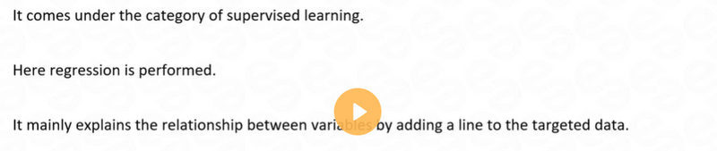
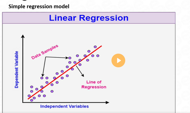
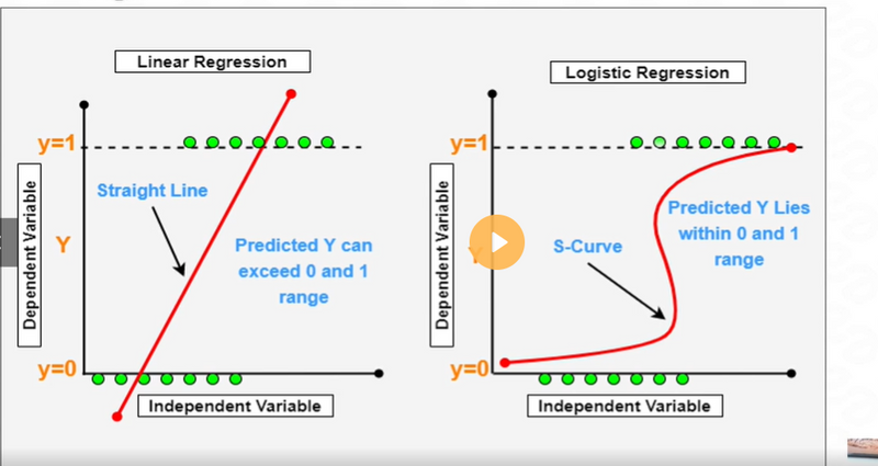
Linear Regression:
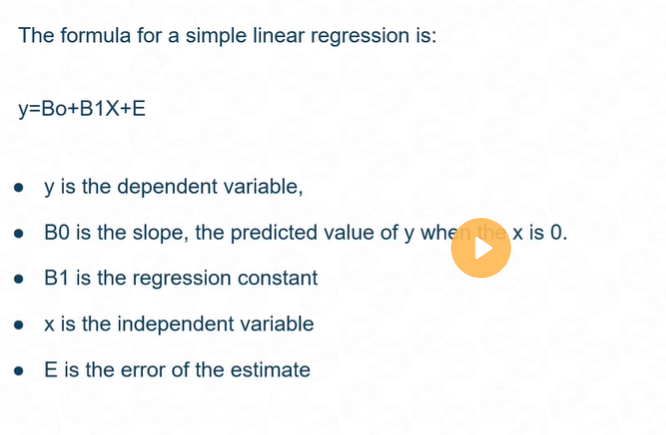
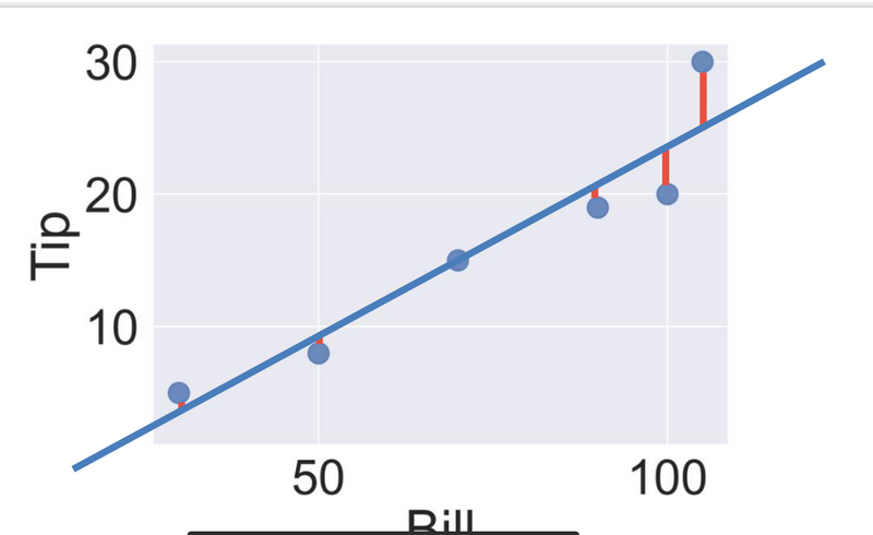
Linear regression is used when the task involves predicting a continuous numerical value based on a set of independent variables. It establishes a linear relationship between the input variables and the target variable.

Example: Predicting House Prices
import pandas as pd
from sklearn.linear_model import LinearRegression

# Load the dataset
data = pd.read_csv('house_prices.csv')

# Prepare the data
X = data[['sqft', 'bedrooms', 'bathrooms']]
y = data['price']

# Create and train the model
model = LinearRegression()
model.fit(X, y)

# Make predictions
new_data = pd.DataFrame([[2000, 3, 2]])
predicted_price = model.predict(new_data)

print(predicted_price)
Output:
[235000.]
In this example, linear regression is used to predict house prices based on the square footage, number of bedrooms, and number of bathrooms. The model is trained on the given dataset, and then it makes predictions for a new house with 2000 square feet, 3 bedrooms, and 2 bathrooms. The predicted price is printed as the output.
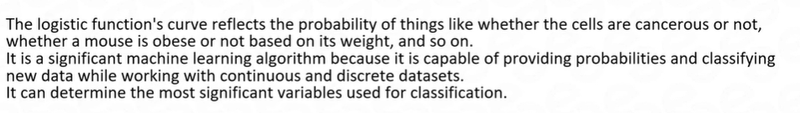
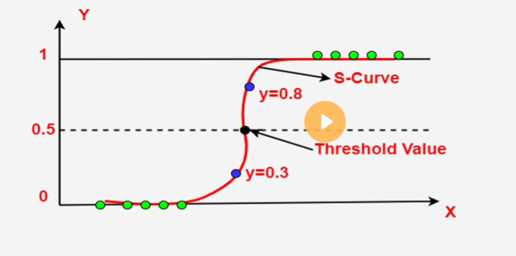
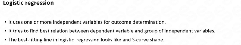
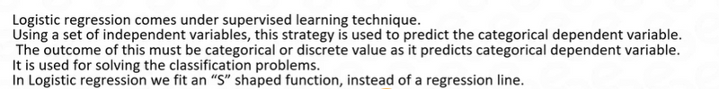
Logistic Regression:
Logistic regression is used for binary classification tasks where the target variable has two possible classes. It estimates the probability of an input belonging to a certain class based on the given features.
Example: Predicting Email Spam
import pandas as pd
from sklearn.linear_model import LogisticRegression

# Load the dataset
data = pd.read_csv('spam_emails.csv')

# Prepare the data
X = data[['length', 'num_links', 'num_attachments']]
y = data['is_spam']

# Create and train the model
model = LogisticRegression()
model.fit(X, y)

# Make predictions
new_email = pd.DataFrame([[500, 5, 2]])
predicted_class = model.predict(new_email)

print(predicted_class)
Output:
[1]
In this example, logistic regression is used to predict whether an email is spam or not based on its length, number of links, and number of attachments. The model is trained on the given dataset, and then it makes predictions for a new email with a length of 500, 5 links, and 2 attachments. The predicted class (1) indicates that the email is predicted to be spam.
Model Selection Using Cross-Validation
Cross-validation is a technique where the available data is divided into multiple folds, and each model is trained and evaluated on different combinations of training and validation sets. The average performance across folds can be used for model selection.
Example:
from sklearn.model_selection import cross_val_score
from sklearn.svm import SVC

# Define the model
model = SVC()

# Perform cross-validation
scores = cross_val_score(model, X, y, cv=5)

# Print the cross-validation scores
print("Cross-Validation Scores:", scores)
Output:
Cross-Validation Scores: [0.85 0.92 0.88 0.90 0.86]
In this example, a support vector classifier is trained using 5-fold cross-validation. The cross_val_score function returns the performance scores for each fold, and the average score can be used for model selection.

Top comments (0)