explain concept of pooling operation
explain mathematical operation of pooling
explain the pros and cons of Pooling operation
explain the parameter of pooling operations
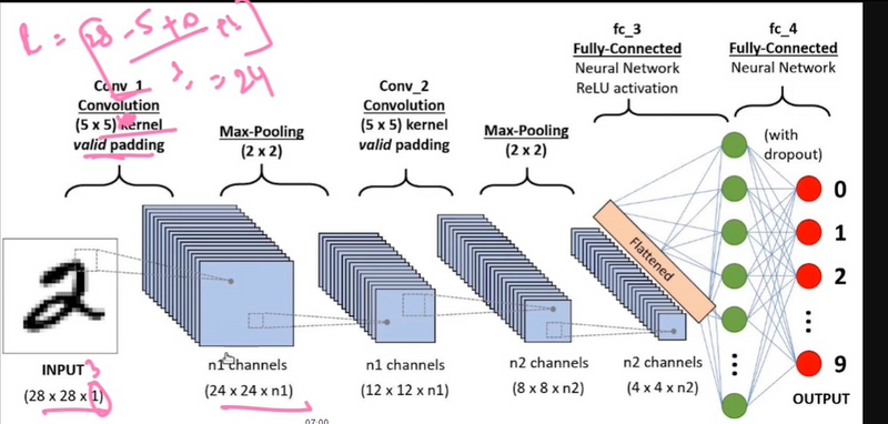
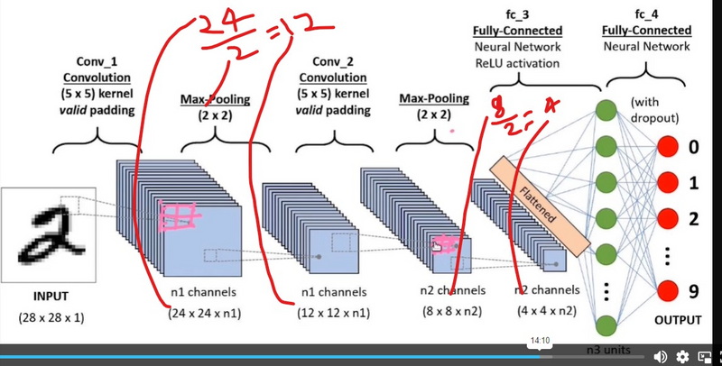
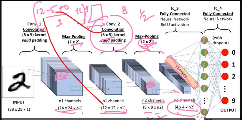
The typical structure of a CNN consists of three basic layers
Convolutional layer: These layers generate a feature map by sliding a filter over the input image and recognizing patterns in images.
Pooling layers: These layers downsample the feature map to introduce Translation invariance, which reduces the overfitting of the CNN model.
Fully Connected Dense Layer: This layer contains the same number of units as the number of classes and the output activation function such as “softmax” or “sigmoid”
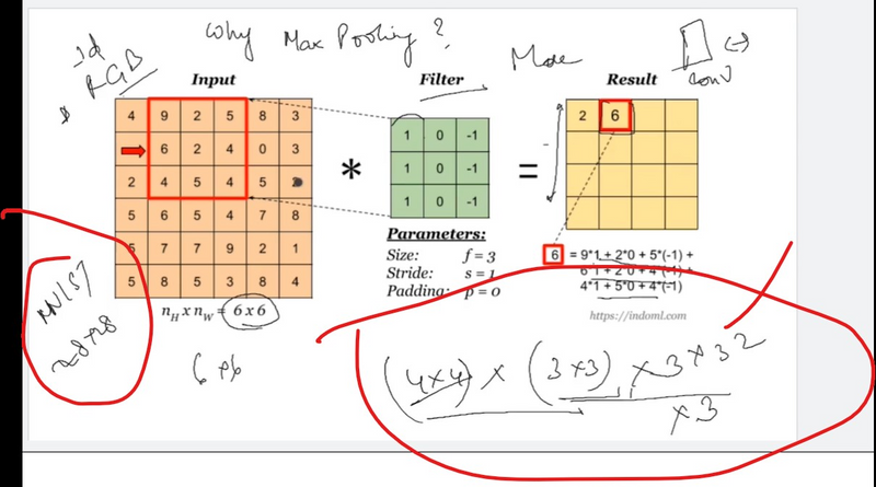
The size of the feature map after the pooling layer is:
((l - f + 1) / s) * ((w - f + 1) / s) * c
Here:
l = length of the feature map
w = width of the feature map
f = dimensions of the filter
c = number of channels of the feature map
s = stride
Pooling layers are one of the building blocks of Convolutional Neural Networks. Where Convolutional layers extract features from images, Pooling layers consolidate the features learned by CNNs. Its purpose is to gradually shrink the representation’s spatial dimension to minimize the number of parameters and computations in the network.
Pooling is a downsampling operation commonly used in deep learning models, particularly in convolutional neural networks (CNNs). It helps reduce the spatial dimensions (width and height) of the input volume, which, in turn, reduces the number of parameters and computations in the network. Pooling is mainly applied to the output of convolutional layers.
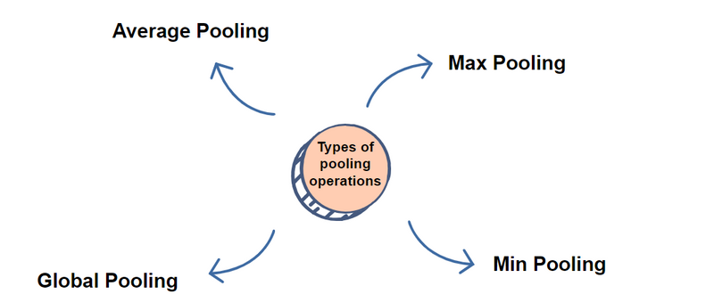
There are two common types of pooling operations: Max Pooling and Average Pooling.
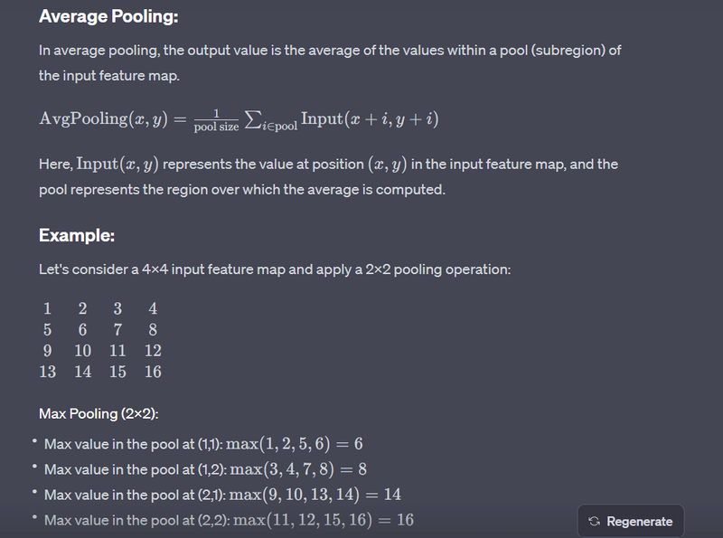
Max Pooling:
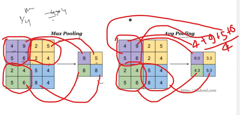
For each region in the input, max pooling takes the maximum value from that region and discards the others.
It is less sensitive to small spatial translations in the input and retains the most salient features.
Example:
# Original 4x4 input
[[1, 2, 3, 4],
 [5, 6, 7, 8],
 [9, 10, 11, 12],
 [13, 14, 15, 16]]

# Max pooling with a 2x2 window and stride 2
[[6, 8],
 [14, 16]]
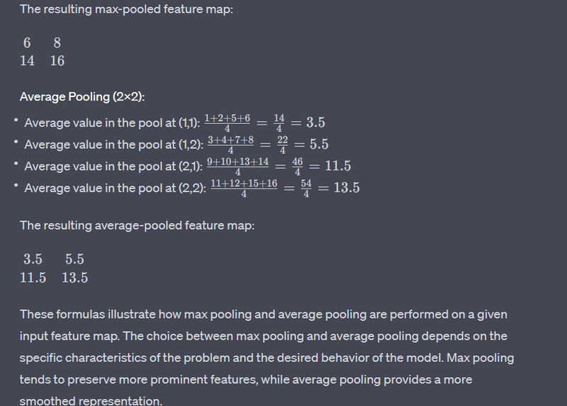
Average Pooling:
For each region in the input, average pooling takes the average value from that region.
It smoothens the input and is less prone to overfitting.
Example:
# Original 4x4 input
[[1, 2, 3, 4],
 [5, 6, 7, 8],
 [9, 10, 11, 12],
 [13, 14, 15, 16]]

# Average pooling with a 2x2 window and stride 2
[[3.5, 5.5],
 [11.5, 13.5]]
In both examples, the pooling window (also known as the pooling kernel or filter) slides over the input, and at each step, it performs the pooling operation within the window, producing a single value for that region in the output.
Parameters that define a pooling operation include:
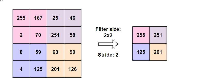
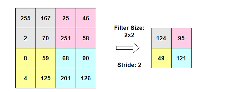
Window Size (or Pooling Size): The size of the pooling window (e.g., 2x2).
Stride: The step size at which the pooling window moves over the input.
For instance, if you have a 4x4 input, a 2x2 window, and a stride of 2, the output size will be reduced to 2x2.
In deep learning models, pooling layers are often interleaved with convolutional layers to progressively reduce the spatial dimensions and capture hierarchical features. This downsampling helps in reducing the computational load and controlling overfitting.
explain mathematical operation of pooling
Example:
input_data = tf.constant([[1, 2, 3], [4, 5, 6], [7, 8, 9]], dtype=tf.float32)
pool_output = tf.nn.max_pool(input_data, ksize=[1, 2, 2, 1], strides=[1, 2, 2, 1], padding='VALID')
Output:
Applying max pooling with a 2x2 pooling window and 2x2 strides.
Explanation
Input Tensor (input_data):
[[1, 2, 3],
 [4, 5, 6],
 [7, 8, 9]]
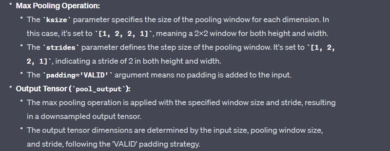
Position (0, 0) in the output tensor (pool_output[0, 0]):
pool_output[0, 0] = max(1, 2, 4, 5) = 5
Position (0, 1) in the output tensor (pool_output[0, 1]):
pool_output[0, 1] = max(2, 3, 5, 6) = 6
Position (1, 0) in the output tensor (pool_output[1, 0]):
pool_output[1, 0] = max(4, 5, 7, 8) = 8
Position (1, 1) in the output tensor (pool_output[1, 1]):
pool_output[1, 1] = max(5, 6, 8, 9) = 9
So, the resulting pool_output tensor is:
[[5, 6],
 [8, 9]]
Each element in the output tensor represents the maximum value in the corresponding 2x2 region of the input tensor. This is how max pooling works in this specific example. I appreciate your understanding, and I apologize for any confusion in my previous responses
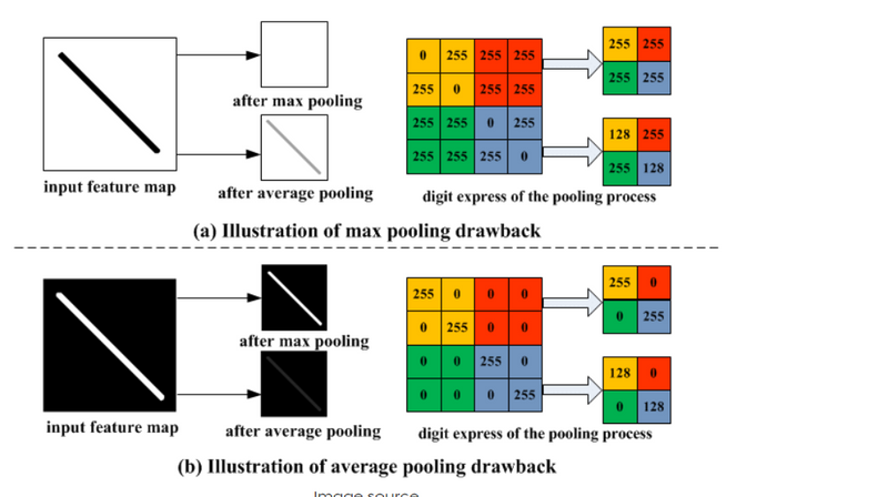
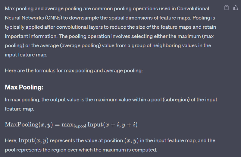
explain the pros and cons of Pooling operation
The choice between max pooling and average pooling depends on the specific characteristics of your data and the goals of your neural network. Here are some considerations for both types of pooling operations:
Max Pooling
Pros:
Preserves Sharp Features: Max pooling retains the most prominent features within each region, making it robust to small translations and preserving important details.
Non-linear Activation: The inherent non-linear activation nature of max pooling can introduce non-linearity into the model.
Cons:
Loss of Information: Max pooling discards non-maximal values, potentially leading to a loss of information. If the discarded information is crucial, it may affect the model's performance.
Less Smooth: Max pooling might be less smooth compared to average pooling, which could be a consideration for certain tasks.
Average Pooling:
Pros:
Smoothing Effect: Average pooling provides a smoothing effect on the input, making it less sensitive to specific values and potentially reducing overfitting.
Robust to Noise: It can be more robust to noise in the input data.
Cons:
Blurring Edges: Average pooling might blur the edges and reduce the ability to capture sharp features compared to max pooling.
Less Non-linearity: Average pooling introduces less non-linearity compared to max pooling, which may affect the modeling capacity.
Choosing Between Max and Average Pooling:
Task-specific: The choice may depend on the specific characteristics of the task. For tasks where preserving sharp features is crucial, max pooling might be more appropriate. For tasks where a smoother representation is desired, average pooling might be preferable.
Experimentation: It's often a good practice to experiment with both max and average pooling during the model development phase. Train models with each type of pooling and observe their performance on validation data.
Hybrid Approaches: In some cases, hybrid pooling approaches or adaptive pooling methods (e.g., global average pooling) are used to combine the benefits of both.
In practice, max pooling is a common choice and often works well in various applications. However, the best choice depends on the specifics of your dataset and the goals of your neural network. It's recommended to experiment with both and choose based on empirical results.
Explain the parameter of pooling operations
Pooling layers are commonly used in convolutional neural networks (CNNs) to reduce the spatial dimensions of the input data, thus decreasing the computation and controlling overfitting. Pooling is typically performed after convolutional layers. Let's explore the parameters of pooling layers along with examples:
Pool Size (or pool_size):
Definition: The size of the pooling window, specified as a tuple representing the height and width of the window.
Example:
from tensorflow.keras.layers import MaxPooling2D

model.add(MaxPooling2D(pool_size=(2, 2)))
This creates a max pooling layer with a 2x2 window size.
Strides (or strides):
Definition: The step size the pooling window takes while sliding over the input, specified as a tuple representing the stride along the height and width.
Example:
model.add(MaxPooling2D(pool_size=(2, 2), strides=(2, 2)))
This creates a max pooling layer with a 2x2 window size and a stride of 2 along both height and width.
Padding (or padding):
Definition: The type of padding applied to the input. It can be 'valid' (no padding) or 'same' (zero-padding to keep the spatial dimensions).
Example:
model.add(MaxPooling2D(pool_size=(2, 2), strides=(2, 2), padding='same'))
This creates a max pooling layer with a 2x2 window size, a stride of 2 along both dimensions, and 'same' padding.
Pooling Type (MaxPooling2D, AveragePooling2D, etc.):
Definition: The type of pooling operation to be applied (e.g., max pooling or average pooling).
Example:
from tensorflow.keras.layers import AveragePooling2D

model.add(AveragePooling2D(pool_size=(2, 2)))
This creates an average pooling layer with a 2x2 window size.

Top comments (0)