Explain the different type of Hyperparameter tuning

Grid Search
brute force approach
Random Search
Bayesian Optimization
Genetic Algorithms
simple imputter

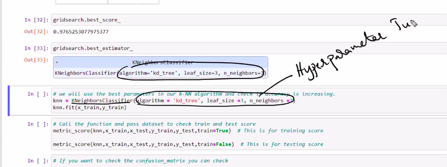
Hyperparameter tuning is the process of finding the best set of hyperparameters for a machine learning model to achieve optimal performance. Hyperparameters are configuration settings that are not learned during the training process but are set before training and can significantly impact the model's performance. There are several methods for hyperparameter tuning, and I'll explain some of the common ones with examples
Grid Search
Grid search involves defining a grid of hyperparameter values and exhaustively searching all possible combinations to find the best set. It's a brute-force approach that can be time-consuming but ensures thorough exploration

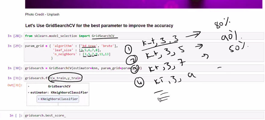
Example: Let's say you have a Support Vector Machine (SVM) model, and you want to tune the C (regularization parameter) and the kernel (linear, polynomial, or radial basis function). You define a grid with various values for C and kernel, and the grid search will train and evaluate the SVM model for each combination of C and kernel to find the best one.

brute force approach

In the context of hyperparameter tuning, the brute force approach involves trying out all possible combinations of hyperparameter values within a predefined range to find the best set of hyperparameters. It is a straightforward and exhaustive method that ensures thorough exploration of the hyperparameter space but can be computationally expensive and time-consuming, especially for models with many hyperparameters or a large range of possible values

Let's illustrate the brute force approach with an example:

Suppose you want to train a k-nearest neighbors (KNN) classifier on a dataset. The KNN algorithm has a hyperparameter called "k," which represents the number of nearest neighbors to consider when making predictions. To tune the "k" hyperparameter using the brute force approach, you would follow these steps

Define the hyperparameter search space: Determine a range of values to explore for the hyperparameter "k." For example, you might decide to try values from 1 to 10.

Evaluate all combinations: Train and evaluate the KNN classifier for each value of "k" within the defined range. This means training the model with k=1, k=2, k=3, and so on, up to k=10.

Select the best hyperparameter: After evaluating the performance of the KNN classifier with different "k" values, choose the value that results in the best performance metric (e.g., accuracy, F1 score, etc.) on a validation set.

Here's a table representing the accuracy of the KNN classifier for different values of "k" during the brute force search:

k (Number of Neighbors) Accuracy
1   0.86
2   0.89
3   0.91
4   0.88
5   0.90
6   0.88
7   0.89
8   0.87
9   0.85
10  0.82

Random Search

Random search samples hyperparameter values randomly from predefined distributions. It is more efficient than grid search for high-dimensional hyperparameter spaces since it explores different combinations with fewer evaluations.

Example: In the same SVM model scenario, instead of defining a grid, you specify distributions for C and randomly sample values from those distributions. For instance, you could sample C from a uniform distribution and the kernel from a list of available options.

Bayesian Optimization

Bayesian optimization uses a probabilistic model to predict the performance of different hyperparameter combinations. It balances exploration and exploitation to efficiently search for the best hyperparameters

Example: Consider a neural network with hyperparameters like learning rate, number of hidden layers, and number of neurons per layer. Bayesian optimization will use the information from previous evaluations to decide which combination to try next and gradually narrow down the search space.

Genetic Algorithms

Genetic algorithms are inspired by natural selection and evolution. It involves creating a population of hyperparameter combinations, evaluating them based on performance, selecting the best ones, and then combining and mutating them to produce the next generation

Example: You have a decision tree classifier with parameters like the maximum depth and minimum number of samples required to split a node. Genetic algorithms will create a population of different parameter sets, evaluate their performance, select the best-performing ones, and perform crossover and mutation to generate the next population.
Gradient-based Optimization

In some cases, hyperparameter tuning can be formulated as an optimization problem itself, and gradient-based methods can be employed to find the optimal values

Example: For some deep learning models, hyperparameters like dropout rate or weight initialization can be tuned using gradient-based optimization techniques like stochastic gradient descent.

These are just a few examples of hyperparameter tuning methods. Depending on the problem and the model, one method may be more suitable than the others. A combination of these methods or using specialized libraries like Optuna, Hyperopt, or scikit-optimize can further enhance the tuning process.

simple imputter

In machine learning, imputing refers to the process of filling in missing values in a dataset. A simple imputer is a basic technique that replaces missing values with a constant or a summary statistic, such as the mean, median, or mode of the non-missing values in the feature. Simple imputers are easy to implement and are a good starting point for handling missing data before exploring more advanced imputation methods.

Let's go through a simple example of using a simple imputer in Python with scikit-learn:

Step 1: Import the necessary libraries

import numpy as np
from sklearn.impute import SimpleImputer

Step 2: Create a sample dataset with missing values
python

data = np.array([[1, 2, 3],
                 [4, np.nan, 6],
                 [7, 8, np.nan],
                 [10, 11, 12]])

In this example, we have a 4x3 array representing a dataset with missing values (indicated by np.nan).

Step 3: Create the SimpleImputer object and specify the imputation strategy

imputer = SimpleImputer(strategy='mean')

Here, we create a SimpleImputer object with the strategy parameter set to 'mean', which means it will replace missing values with the mean of the non-missing values along each column.

Step 4: Fit the imputer to the data and transform the dataset

imputer.fit(data)
imputed_data = imputer.transform(data)

The fit method computes the mean of each column and stores it in the imputer object. The transform method replaces the missing values in the dataset with the corresponding means.

Step 5: Display the imputed dataset

print("Original Data:\n", data)
print("Imputed Data:\n", imputed_data)

Output:

Original Data:

 [[ 1.  2.  3.]
 [ 4. nan  6.]
 [ 7.  8. nan]
 [10. 11. 12.]]

Imputed Data:

 [[ 1.   2.   3. ]
 [ 4.   7.  6. ]
 [ 7.   8.  7. ]
 [10.  11. 12. ]]

As you can see, the missing values in the original dataset have been replaced by the mean of the corresponding columns. In the second row, the missing value in the second column (previously np.nan) is now replaced by the mean of the second column, which is (2 + 8 + 11) / 3 = 7.

Simple imputers can be a useful first step in handling missing data, but they may not be suitable for all datasets or situations. Other imputation techniques, such as K-nearest neighbors imputation, regression imputation, or iterative imputation, can be explored when dealing with more complex data or datasets with high levels of missingness.