Explain the Fast RCNN Architecture in Deep learning

Need for Fast RCNN
Model architecture of Fast RCNN
Why we need ROI pooling layer in Fast RCNN
pros and cons of fast RCNN

Need for Fast RCNN

1. The training of R-CNN is very slow because each part of the model such as (CNN, SVM classifier, and bounding box) requires training separately and cannot be paralleled.
2. Also, in R-CNN we need to forward and pass every region proposal through the Deep Convolution architecture (that’s up to ~2000 region proposals per image). That explains the amount of time taken to train this model
3. The testing time of inference is also very high. It takes 49 seconds to test an image in R-CNN (along with selective search region proposal generation)

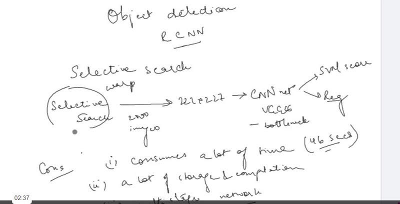
R-CNN: R-CNN was proposed by Ross Girshick et al. in 2014 to deal with the problem of efficient object localization in object detection. The previous methods use what is called Exhaustive Search which uses sliding windows of different scales on image to propose region proposals Instead, this paper uses the Selective search algorithm which takes advantage of segmentation of objects and Exhaustive search to efficiently determine the region proposals. This selective search algorithm proposes approximately 2000 region proposals per image. These are then passed to the CNN model (Here AlexNet is used).

1. AlexNet is a convolutional neural network (CNN) architecture that was developed by Alex Krizhevsky, Ilya Sutskever, and Geoffrey Hinton in 2012. It was the first CNN to win the ImageNet Large Scale Visual Recognition Challenge (ILSVRC), a major image recognition competition, and it helped to establish CNNs as a powerful tool for image recognition.
2. AlexNet consists of several layers of convolutional and pooling layers, followed by fully connected layers. The architecture includes five convolutional layers, three pooling layers, and three fully connected layers.
3. The first two convolutional layers use a kernel of size 11×11 and apply 96 filters to the input image. The third and fourth convolutional layers use a kernel of size 5×5 and apply 256 filters. The fifth convolutional layer uses a kernel of size 3×3 and applies 384 filters. The output of these convolutional layers is then passed through max-pooling layers that reduce the spatial dimensions of the feature maps.
4. The output of the pooling layers is then passed through three fully connected layers, with 4096, 4096, and 1000 neurons respectively. The last fully connected layer is used for classification, and produces a probability distribution over the 1000 ImageNet classes.
5. AlexNet was trained on the ImageNet dataset, which consists of 1.2 million images with 1000 classes, and was able to achieve high recognition accuracy. The AlexNet architecture was the first to show that CNNs could significantly outperform traditional machine learning methods in image recognition tasks, and was an important step in the development of deeper architectures like VGGNet, GoogleNet, and ResNet .

This CNN model then outputs a (1, 4096) feature vector from each region proposal. This vector then passed into the SVM model for classification of object and bounding box regressor for localization. Problem with R-CNN:

1. Each image needs to classify 2000 region proposals. So, it takes a lot of time to train the network.
2. It requires 49 seconds to detect the objects in an image on GPU.
3. To store the feature map of the region proposal, lots of Disk space is also required.

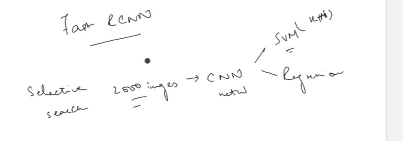
Fast R-CNN : In R-CNN we passed each region proposal one by one in the CNN architecture and selective search generated around 2000 region proposal for an image. So, it is computationally expensive to train and even test the image using R-CNN. To deal with this problem Fast R-CNN was proposed, It takes the whole image and region proposals as input in its CNN architecture in one forward propagation. It also combines different parts of architecture (such as ConvNet, RoI pooling, and classification layer) in one complete architecture. That also removes the requirement to store a feature map and saves disk space. It also uses the softmax layer instead of SVM in its classification of region proposal which proved to be faster and generate better accuracy than SVM.

The network is modified in such a way that it two inputs the image and list of region proposals generated on that image.
Second, the last pooling layer (here (7*7*512)) before fully connected layers needs to be replaced by the region of interest (RoI) pooling layer.
Third, the last fully connected layer and softmax layer is replaced by twin layers of softmax classifier and K+1 category-specific bounding box regressor with a fully connected layer.
Multi-stage, expensive training: The separate training processes required for all the stages of the network — fine-tuning a CNN on object proposals, learning an SVM to classify the feature vector of each proposal from the CNN and learning a bounding box regressor to fine-tune the object proposals (refer to Regions with CNNs for more details) proves to be a burden in terms of time, computation and resources. For example, to train the SVM, we would need the features of thousands of possible region proposals to be written to the disk from the previous stage.
Slow test time: Given this multi-stage pipeline, detection using a simple VGG network as the backbone CNN takes 47s/image.

Model architecture of Fast RCNN

Architecture details:
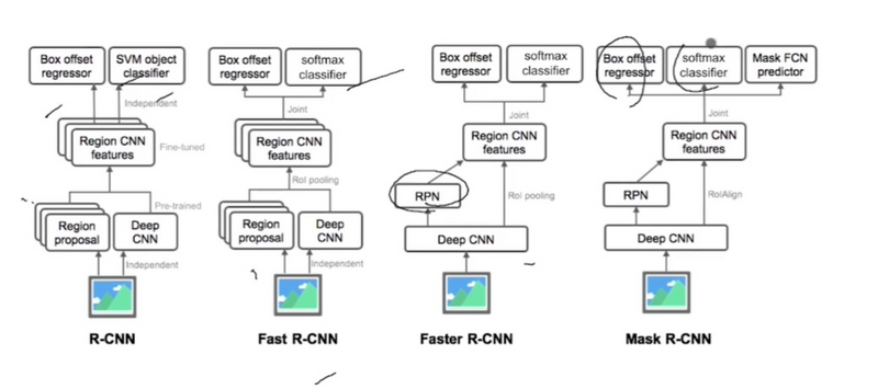
To better understand how and why the Fast R-CNN improved efficiency and performance of R-CNN and SPP Networks, let’s first look into its architecture.

1.The Fast R-CNN consists of a CNN (usually pre-trained on the ImageNet classification task) with its final pooling layer replaced by an “ROI pooling” layer and its final FC layer is replaced by two branches — a (K + 1) category softmax layer branch and a category-specific bounding box regression branch.

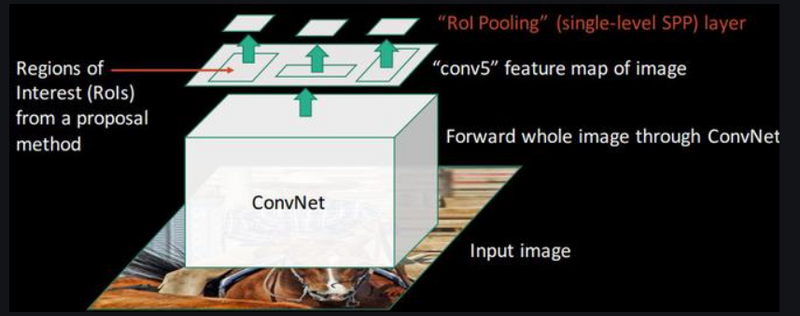
Figure 1: The Fast R-CNN pipeline

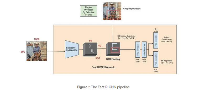
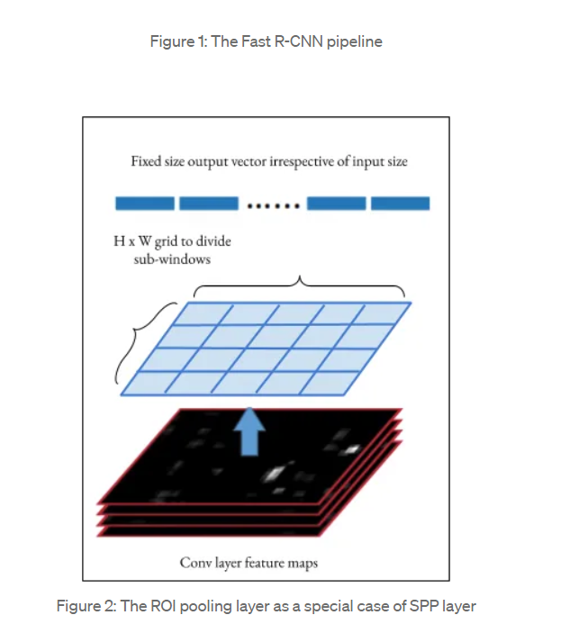
Figure 2: The ROI pooling layer as a special case of SPP layer
1.The entire image is fed into the backbone CNN and the features from the last convolution layer are obtained. Depending on the backbone CNN used, the output feature maps are much smaller than the original image size. This depends on the stride of the backbone CNN, which is usually 16 in the case of a VGG backbone.

2.Meanwhile, the object proposal windows are obtained from a region proposal algorithm like selective search[4]. As explained in Regions with CNNs, object proposals are rectangular regions on the image that signify the presence of an object.
The portion of the backbone feature map that belongs to this window is then fed into the ROI Pooling layer.
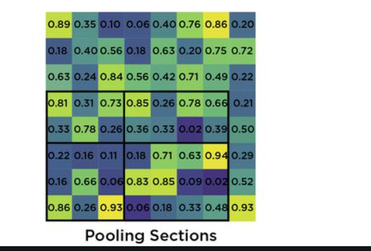
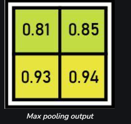
3.The ROI pooling layer is a special case of the spatial pyramid pooling (SPP) layer with just one pyramid level. The layer basically divides the features from the selected proposal windows (that come from the region proposal algorithm) into sub-windows of size h/H by w/W and performs a pooling operation in each of these sub-windows. This gives rise to fixed-size output features of size (H x W) irrespective of the input size. H and W are chosen such that the output is compatible with the network’s first fully-connected layer. The chosen values of H and W in the Fast R-CNN paper is 7. Like regular pooling, ROI pooling is carried out in every channel individually.

4.The output features from the ROI Pooling layer (N x 7 x 7 x 512 where N is the number of proposals) are then fed into the successive FC layers, and the softmax and BB-regression branches. The softmax classification branch produces probability values of each ROI belonging to K categories and one catch-all background category. The BB regression branch output is used to make the bounding boxes from the region proposal algorithm more precise

Why we need ROI pooling layer in Fast RCNN

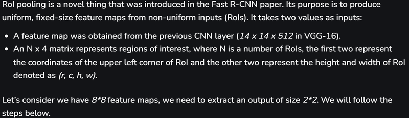
In Fast R-CNN, the input to the network is a convolutional feature map of the entire image. Since different ROIs can have different sizes and aspect ratios, directly feeding them into a fully connected layer would require fixed-size inputs, which is impractical

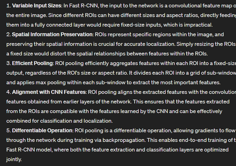
Overall, the ROI pooling layer in Fast R-CNN enables efficient extraction of fixed-size feature representations from variable-sized ROIs while preserving spatial information, thereby facilitating accurate object detection and localization

pros and cons of fast RCNN

Pros

Improved Speed: Fast R-CNN introduced several optimizations, such as the Region of Interest (ROI) pooling layer and sharing convolutional features across multiple regions, leading to faster inference compared to R-CNN. This speed improvement makes it more practical for real-time or near-real-time applications.
End-to-End Training: Unlike R-CNN, which involved training separate models for region proposal and object detection, Fast R-CNN enables end-to-end training. This simplifies the training process, reduces the need for multiple stages of training, and potentially improves performance.
Better Localization Accuracy: By utilizing the ROI pooling layer, which preserves spatial information within regions of interest, Fast R-CNN achieves better localization accuracy compared to methods that directly resize regions to a fixed size.
Flexibility in CNN Architectures: Fast R-CNN is compatible with various CNN architectures for feature extraction, allowing researchers to leverage the latest advancements in deep learning architectures to improve object detection performance.
Single Model for Region Proposal and Detection: Fast R-CNN integrates region proposal and object detection into a single model, eliminating the need for separate algorithms for these tasks. This simplifies the overall architecture and reduces computational overhead.

Cons

:

Computational Complexity: While Fast R-CNN is faster than its predecessor, it still involves significant computational complexity, particularly during training. Generating region proposals, extracting features, and performing classification and regression for each region require substantial computational resources.
Training Data Dependency: Fast R-CNN's performance heavily depends on the availability and quality of training data, particularly annotated datasets with bounding box labels. Limited or biased training data can lead to suboptimal performance and generalization issues.
Memory Consumption: Training Fast R-CNN models requires large amounts of GPU memory due to the need to store intermediate feature representations for each region proposal. This can limit the model's scalability and practicality on resource-constrained systems.
Architecture Complexity: While Fast R-CNN simplified the training pipeline compared to R-CNN, it still has a complex architecture with multiple components, including region proposal generation, feature extraction, and classification/regression. This complexity can make it challenging to understand, implement, and optimize.
Fine-tuning Challenges: Fine-tuning pre-trained Fast R-CNN models for specific tasks or domains may require careful adjustment of hyperparameters and architectural modifications to achieve optimal performance. This process can be time-consuming and resource-intensive.

.