Section 1 — Training / Model Creation
Section 2 — Inference / Actual LLM Processing
LLM Foundations Experiment Lab
Experiments to Build
Recommended Final Mini-Projects
Final Project — LLM Foundations Experiment Lab
Most Important Experiments
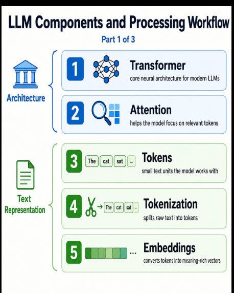
LLM Architecture is the internal structure and flow of a Large Language Model that explains how it takes text as input, understands context, and generates the next words as output.
In simple flow:
Input Text → Tokens → Embeddings → Transformer → Attention → Context Understanding → Next-Token Prediction → Output Text
Example:
Input: “The cat is sitting on the…”
The LLM processes the words using tokens, embeddings, transformers, and attention, then predicts:
Output: “mat”
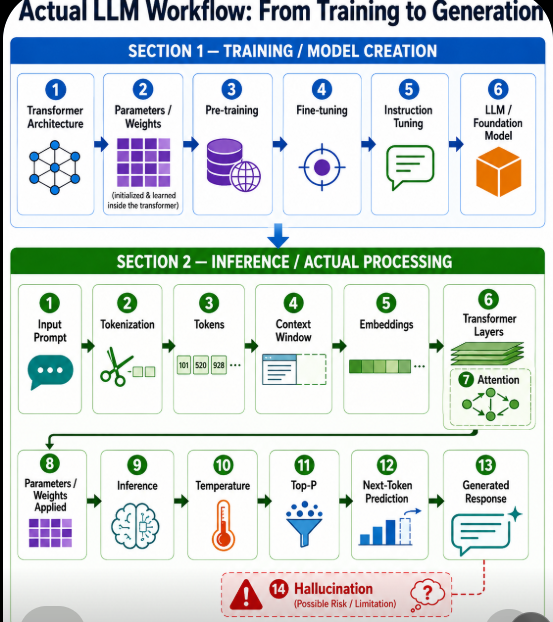
Section 1: how an LLM is created/trained.
Section 2: what happens when a user actually sends a prompt.
Section 1 — Training / Model Creation
These steps happen before you use ChatGPT-like models.
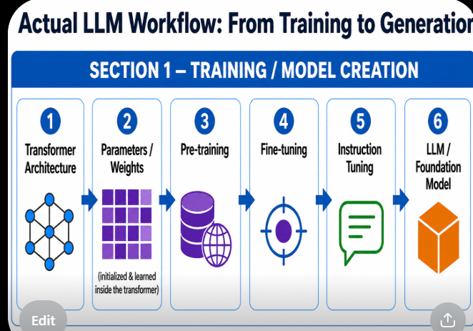
Section 1 in one line
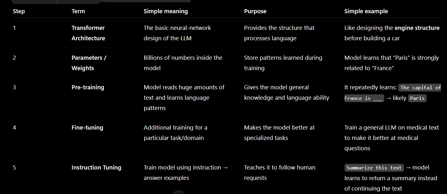
Transformer Architecture
↓
Initialize Parameters
↓
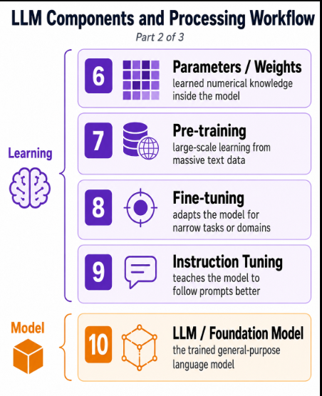
Pre-training learns general patterns
↓
Optional Fine-tuning
↓
Instruction Tuning
↓
Trained LLM
Section 2 — Inference / Actual LLM Processing
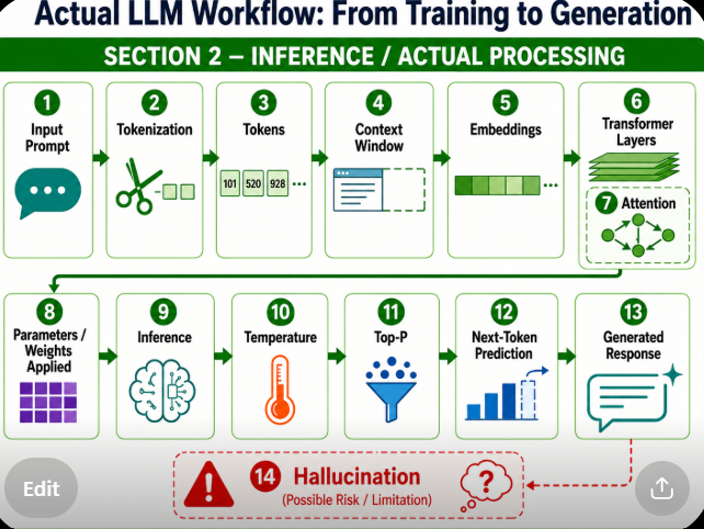
Now suppose you type:
“Explain photosynthesis in simple words.”
This is where actual runtime processing starts.
- Input Prompt
Explain photosynthesis in simple words.
This is simply the text sent by the user.
Purpose: Tell the LLM what you want.
- Tokenization
The model cannot directly work with normal sentences. A tokenizer breaks text into smaller pieces.
For example, conceptually:
"Explain photosynthesis in simple words."
↓ Tokenization
["Explain", " photo", "synthesis", " in", " simple", " words", "."]
Real tokenizers may split words differently.
Purpose: Convert human text into units the model can process.
- Tokens
Each token is represented by a numerical ID.
For example:
Explain → 21435
photo → 9821
synthesis → 17420
in → 287
simple → 4382
words → 2456
So:
Text
↓
Tokenization
↓
Tokens
↓
[21435, 9821, 17420, 287, 4382, 2456]
Purpose: Give every text piece a machine-readable identity.
- Context Window
The context window defines how many tokens the LLM can consider together.
Imagine the model can process:
Previous conversation
+
System instructions
+
User prompt
+
Retrieved information
all within its available context.
Conceptually:
┌──────────── Context Window ───────────────┐
│ Previous conversation │
│ User: What is a plant? │
│ Assistant: ... │
│ User: Explain photosynthesis simply │
└──────────────────────────────────────────┘
Purpose: Determines how much information the model can use while answering.
A small correction to your diagram: context window isn't really a transformation step like tokenization or embeddings. It is better thought of as the limit/boundary around the tokens being processed.
- Embeddings
Token IDs such as:
21435
9821
17420
don't contain useful meaning by themselves.
The model converts them into vectors:
"plant"
↓
[0.21, -0.54, 0.88, 0.13, ...]
"sunlight"
↓
[0.17, -0.49, 0.91, 0.08, ...]
These vector representations allow the neural network to work with language mathematically.
Purpose: Convert token IDs into numerical representations that the Transformer can process.
So:
Text
↓
Tokenization
↓
Tokens / Token IDs
↓
Embeddings
Transformer Layers
Now the embeddings enter many Transformer layers.
Conceptually:
Embeddings
↓
Transformer Layer 1
↓
Transformer Layer 2
↓
Transformer Layer 3
↓
...
↓
Transformer Layer N
Every layer improves the model's representation of the text.
For our example:
Explain photosynthesis in simple words
The model gradually understands relationships involving:
photosynthesis
sunlight
plants
water
carbon dioxide
oxygen
Purpose: Perform the main language reasoning/processing.
- Attention
Attention happens inside Transformer layers.
This is extremely important.
For example:
“The plant uses sunlight to make its food.”
While processing the word “its”, attention can connect it strongly with:
plant
rather than:
sunlight
Simplified:
The plant uses sunlight to make its food
↑ ↑
└──────── Attention ──────┘
For your photosynthesis prompt, attention may establish relationships like:
photosynthesis
↓
sunlight
↓
plant
↓
water
↓
carbon dioxide
Purpose: Determine which other tokens are relevant to the token currently being processed.
So the correct relationship is:
Transformer Layer
│
├── Attention
├── Feed-Forward Network
├── Normalization
└── Residual Connections
Attention is not outside the Transformer. It is one of its core mechanisms.
- Parameters / Weights Applied
Remember the billions of weights learned during training?
They are now used throughout the Transformer calculations.
For example, during training the model may have learned strong patterns involving:
photosynthesis ↔ plants
photosynthesis ↔ sunlight
photosynthesis ↔ carbon dioxide
photosynthesis ↔ oxygen
Those learned relationships influence its processing.
Purpose: Apply previously learned knowledge/patterns.
But technically, your diagram simplifies this. Parameters aren't really a separate step after Attention.
A more accurate view is:
Learned Parameters
↓
Embeddings → Transformer Layers → Output
↑
Attention
The weights operate throughout the Transformer.
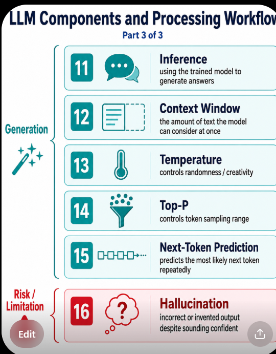
- Inference
Inference means:
Using the already-trained model to answer a new request.
Everything happening after you submit:
Explain photosynthesis in simple words.
is inference.
Therefore inference is actually the name of the whole runtime process, not just one small processing box.
Think:
Training
= Learning
Inference
= Using what was learned
Example:
TRAINING:
Read millions of science documents
INFERENCE:
User asks:
"What is photosynthesis?"
Model generates an answer
- Next-Token Prediction
Ultimately, an autoregressive LLM repeatedly predicts the next token.
Suppose it has started:
Photosynthesis is the process by which plants...
The model computes probabilities for possible next tokens:
use 45%
make 20%
convert 15%
absorb 10%
other 10%
One token is selected.
Then:
Photosynthesis is the process by which plants use
Now the model predicts again:
sunlight 70%
water 10%
energy 8%
food 5%
Select one:
sunlight
Then repeat.
Photosynthesis
↓
Photosynthesis is
↓
Photosynthesis is the
↓
Photosynthesis is the process
↓
Purpose: Generate the response token by token.
- Temperature
Temperature changes how adventurous/random token selection is.
Imagine:
Next-token probabilities:
sunlight 70%
energy 15%
water 8%
light 5%
other 2%
Low temperature
Model strongly favors high-probability choices.
sunlight
Usually gives:
more predictable
more focused
more consistent output
Higher temperature
Lower-probability tokens have a greater chance.
This can produce:
more variety
more creativity
sometimes more mistakes
Purpose: Control randomness during generation.
- Top-P
Top-P is another token-sampling control.
Suppose:
sunlight 50%
light 20%
energy 15%
water 8%
plants 4%
other 3%
With:
Top-P = 0.90
the sampler considers enough high-probability tokens to reach roughly 90% cumulative probability.
Conceptually:
sunlight 50%
+
light 20%
+
energy 15%
+
water 8%
-------------
93%
Lower-probability alternatives outside that selected probability mass can be excluded.
Purpose: Control how broad the candidate token pool is.
- Generated Response
After repeating next-token generation many times:
Token 1
↓
Token 2
↓
Token 3
↓
Token 4
↓
you finally see something like:
Photosynthesis is the process plants use to make food. They use sunlight, water, and carbon dioxide to produce glucose and release oxygen.
That is the generated response.
- Hallucination
Hallucination is not a processing step.
It is a possible failure mode of the generated response.
For example, imagine the LLM says:
“Plants perform photosynthesis mainly using oxygen.”
That would be incorrect.
The output may sound confident even though the information is wrong.
So your diagram correctly puts Hallucination separately as:
Generated Answer
│
└──── Possible Risk
↓
Hallucination
Purpose in the diagram: Show an important limitation/risk of LLM generation.
The actual flow to remember
For learning LLM processing, I recommend remembering it like this:
USER PROMPT
↓
Tokenization
↓
Tokens
↓
Embeddings
↓
┌─────────────────────────┐
│ TRANSFORMER LAYERS │
│ │
│ Attention │
│ + │
│ Learned Weights │
│ + │
│ Feed-Forward Network │
│ + │
│ Other Components │
└────────────┬────────────┘
↓
Output Scores
/ Logits
↓
Token Probabilities
↓
Temperature + Top-P
↓
Select Next Token
↓
Add Token to the Context
↓
Run Model Again
↓
REPEAT
↓
Generated Answer
│
└── Possible Hallucination
┌──────────────── CONTEXT WINDOW ────────────────┐
│ │
│ User Prompt + Previous Tokens + Generated Text │
│ │
└────────────────────────────────────────────────┘
One correction that makes your diagram much more technically accurate
Instead of remembering:
Inference
↓
Temperature
↓
Top-P
↓
Next-Token Prediction
remember:
Transformer Processing
↓
Next-Token Scores / Logits
↓
Probabilities
↓
Temperature / Top-P
↓
Select Next Token
↓
Append Token
↓
Repeat Transformer Processing
LLM Foundations Experiment Lab
Goal
Build one learning project that allows you to see what is happening inside an LLM, instead of treating the model like a black box.
User Prompt
↓
Tokenization
↓
Tokens / Token IDs
↓
Embeddings
↓
Transformer Layers
├── Self-Attention
├── Q / K / V
├── Feed-Forward Network
├── Residual Connections
└── Normalization
↓
Hidden Representation
↓
Logits
↓
Probabilities
↓
Temperature
↓
Top-P
↓
Select Next Token
↓
Append Token to Context
↓
Run Transformer Again
↓
REPEAT
↓
Generated Response
Possible Failure
↓
Hallucination
This follows the main inference workflow described in the blog.
Experiments to Build
- Experiment 1 — Prompt Input Inspector
Enter different prompts.
Print the raw prompt.
Print character count.
Print word count.
Later compare these numbers with token count.
-
Example:
Explain photosynthesis in simple words. Learn: Prompt, input text, inference request.
- Experiment 2 — Tokenization Explorer
- Pass the same sentence through a real tokenizer.
- Display each individual token.
-
Try:
cat cats unbelievable photosynthesis AI Agentic AI MyHospitalNow Compare normal words, rare words, punctuation and numbers.
Learn: Tokenization, subword tokens, tokenizer vocabulary.
Tokenizers convert text into model inputs and may split uncommon words into smaller subword units.
- Experiment 3 — Token → Token ID Explorer
-
Display:
Token Token ID -------------------------------- Explain 1234 photo 5678 synthesis 9123 Decode every ID back to its token.
-
Verify:
Text ↓ Tokens ↓ IDs ↓ Tokens ↓ Text Learn: Vocabulary and machine-readable token identities.
- Experiment 4 — Token Count / Context Window Lab
-
Generate prompts of:
- 10 tokens
- 100 tokens
- 500 tokens
- 1,000+ tokens
-
Display:
Context used: 812 tokens Context limit: .... Remaining capacity: .... Add conversation history and observe token growth.
Learn: Context window, conversation history, prompt size.
The context window should be understood as the boundary around the tokens being processed rather than another neural transformation step.
- Experiment 5 — Embedding Vector Inspector
Take token IDs and retrieve their input embeddings.
-
Display a shortened version:
"plant" ↓ [0.21, -0.54, 0.88, ...] "sunlight" ↓ [0.17, -0.49, 0.91, ...] -
Print:
Token Token ID Embedding dimensions First 10 vector values Learn: Embeddings, vectors, dimensions.
- Experiment 6 — Embedding Similarity Experiment
-
Compare representations for words such as:
doctor physician car vehicle king banana Calculate cosine similarity where appropriate.
Important: distinguish the model's input token embeddings from sentence/document embeddings used in semantic search.
Learn: Vector representations and similarity.
- Experiment 7 — Position Information Experiment
-
Compare:
Dog bites man. Man bites dog. Tokens may be similar while their ordering changes the meaning.
Inspect how the model represents positions according to the architecture being used.
Learn: Why sequence position matters.
- Experiment 8 — Transformer Layer Inspector
-
Run:
The animal didn't cross the street because it was tired. Retrieve hidden states from each Transformer layer.
-
Display:
Embedding representation ↓ Layer 1 representation ↓ Layer 2 representation ↓ Layer 3 representation ↓ ... Final representation Compare how a token's vector changes between layers.
Learn: Transformer processing and contextual representations.
Transformer model outputs can expose hidden states from successive layers for inspection.
- Experiment 9 — Self-Attention Visualization
-
Use:
The animal didn't cross the street because it was tired. Select the token representing "it".
Visualize which previous tokens receive attention.
-
Produce an attention heatmap:
animal street because it tired it ████ ░ ░ █ ██ Learn: Attention and token relationships.
Attention weights can be returned by supported Transformer model outputs for analysis.
- Experiment 10 — Query, Key and Value Lab
* Build a tiny self-attention calculation manually.
* Show:
```text
Current token
↓
Query
Other tokens
↓
Keys
Query × Keys
↓
Attention scores
↓
Softmax
↓
Attention weights
Attention weights × Values
↓
Contextual representation
```
* Use very small vectors such as 3–4 dimensions.
* **Learn:** Q, K, V and how self-attention is calculated.
- Experiment 11 — Multi-Head Attention Explorer
* Inspect several attention heads.
* Compare whether different heads emphasize different token relationships.
* Display:
```text
Layer 3
├── Head 1
├── Head 2
├── Head 3
└── Head 4
```
* **Learn:** Multi-head attention.
- Experiment 12 — Feed-Forward + Residual + Normalization Lab
* Build a miniature Transformer block.
* Show conceptually:
```text
Input
↓
Self-Attention
↓
Residual Connection
↓
Normalization
↓
Feed-Forward Network
↓
Residual Connection
↓
Normalization
```
* Print tensor shapes after each operation.
* **Learn:** Attention is only one component of a Transformer block.
The blog likewise places attention, feed-forward processing, normalization and residual connections inside Transformer processing.
- Experiment 13 — Model Parameters Inspector
* Print:
```text
Model parameters
Trainable parameters
Frozen parameters
Embedding parameters
Transformer-layer parameters
Output-head parameters
```
* Inspect several actual weight matrices.
* **Learn:** Parameters/weights and where learned information resides.
- Experiment 14 — Random Model vs Pretrained Model
* Initialize the same architecture with random parameters.
* Give it:
```text
Paris is the capital of
```
* Compare against the pretrained version.
* Expected learning result:
```text
Random parameters
↓
meaningless predictions
Learned parameters
↓
useful language predictions
```
* **Learn:** Why pre-training matters.
- Experiment 15 — Tiny Pre-training Experiment
* Do **not** try to train a real billion-parameter LLM.
* Create a tiny Transformer language model.
* Train it on a tiny text corpus.
* Record:
```text
Epoch
Loss
Next-token accuracy/example predictions
```
* Compare predictions before and after training.
* **Learn:** Pre-training, loss, optimization, parameter updates.
- Experiment 16 — Fine-Tuning Experiment
* Start with a pretrained causal language model.
* Fine-tune it on a tiny domain dataset such as:
```text
Hospital FAQs
Travel FAQs
DevOps questions
Product documentation
```
* Compare:
```text
Base Model
VS
Fine-Tuned Model
```
* **Learn:** Fine-tuning and domain adaptation.
Hugging Face provides an official causal-language-modeling workflow showing training/fine-tuning and subsequent generation.
- Experiment 17 — Instruction-Tuning Concept Lab
* Prepare examples such as:
```text
Instruction:
Explain Docker simply.
Response:
Docker packages an application...
```
* Compare ordinary continuation data:
```text
Docker is...
```
against instruction-response data:
```text
User: Explain Docker simply.
Assistant: ...
```
* **Learn:** Difference between pre-training data and instruction-style training data.
- Experiment 18 — Inference Inspector
* Put the model in inference/evaluation mode.
* Submit a new prompt.
* Ensure no training or parameter update occurs.
* Display:
```text
TRAINING
Data → Loss → Backpropagation → Update weights
INFERENCE
Prompt → Existing weights → Prediction
```
* **Learn:** Training vs inference.
- Experiment 19 — Logits Inspector
* Enter:
```text
The capital of France is
```
* Run one forward pass.
* Inspect output logits for the final position.
* Display top candidate tokens:
```text
Token Logit
-----------------
Paris ...
Lyon ...
France ...
London ...
```
* **Learn:** Logits / raw next-token scores.
Model outputs expose logits, making this stage directly inspectable.
- Experiment 20 — Logits → Probability Experiment
* Apply softmax manually.
```text
Logits
↓
Softmax
↓
Probabilities
Paris 72%
Lyon 8%
London 4%
...
```
* Confirm probabilities sum approximately to 1.
* **Learn:** How output scores become candidate probabilities.
- Experiment 21 — Greedy Next-Token Predictor
* Select the token with the highest probability.
```text
Prompt
↓
Model
↓
Logits
↓
Softmax
↓
Highest probability
↓
Next token
```
* Print the top 10 candidates each time.
* **Learn:** Next-token prediction.
- Experiment 22 — Temperature Lab
* Generate the same prompt repeatedly:
```text
AI will change software development by
```
* Test several temperature settings.
* Compare:
```text
Lower temperature → generally more concentrated sampling
Higher temperature → generally more diverse sampling
```
* Save every output for comparison.
* **Learn:** Temperature and randomness.
Generation APIs expose temperature as one of the decoding controls.
- Experiment 23 — Top-P Lab
* Take candidate probabilities:
```text
A 40%
B 25%
C 15%
D 10%
E 5%
F 5%
```
* Manually calculate the nucleus retained by different `top_p` settings.
* Then test generation with those settings.
* **Learn:** Nucleus sampling / Top-P.
Top-P keeps a sufficiently probable candidate set whose cumulative probability reaches the configured threshold.
- Experiment 24 — Temperature vs Top-P Comparison
* Hold one constant while varying the other.
* Record:
```text
Prompt
Temperature
Top-P
Output
Repetition
Diversity
```
* **Learn:** These parameters influence sampling in different ways.
- Experiment 25 — Manual Autoregressive Generation Loop
* This is one of the **most important experiments**.
Implement:
```text
Prompt
↓
Tokenize
↓
Transformer
↓
Logits for last position
↓
Probabilities
↓
Sample next token
↓
Append token
↓
Feed enlarged sequence back into model
↓
Predict again
↓
REPEAT
```
* Do **not** initially use the high-level `generate()` method.
* Write the loop yourself.
* Print:
```text
Step 1
Context: "AI is"
Predicted: "changing"
Step 2
Context: "AI is changing"
Predicted: "the"
Step 3
Context: "AI is changing the"
Predicted: "world"
```
* **Learn:** Autoregressive generation.
The blog identifies this repeating append-and-run-again loop as the central idea behind autoregressive text generation.
- Experiment 26 — Context Growth Visualizer
* Extend Experiment 25.
* Display:
```text
Step 0:
[The] [cat]
Step 1:
[The] [cat] [is]
Step 2:
[The] [cat] [is] [sitting]
Step 3:
[The] [cat] [is] [sitting] [on]
Step 4:
[The] [cat] [is] [sitting] [on] [the]
```
* Display token count after every generation step.
* **Learn:** Generated tokens become part of subsequent context.
- Experiment 27 — Prompt Sensitivity Experiment
* Compare:
```text
Explain Transformer.
Explain Transformer simply.
Explain Transformer to a 10-year-old.
Explain Transformer to a senior AI engineer.
```
* Compare generated tokens and answers.
* **Learn:** Context changes probability distributions and output.
- Experiment 28 — Previous Conversation Context Experiment
* Try:
```text
User: My favorite language is Python.
Assistant: Understood.
User: Which language did I mention?
```
* Then remove the previous context.
* Compare.
* **Learn:** Context-window information versus model parameters.
- Experiment 29 — Hallucination Lab
* Ask questions about deliberately fictional entities or unavailable facts.
* Record whether the model:
* admits uncertainty,
* gives unsupported information,
* invents details.
* Compare different prompts.
* **Learn:** Hallucination as a generation failure rather than a Transformer processing stage.
That distinction matches the blog: hallucination appears after generation as a possible risk, not as part of the forward-processing pipeline.
- Experiment 30 — Full LLM Workflow Visualizer
* Combine all previous experiments into one application.
User enters:
```text
The cat is sitting on the
```
Application displays:
```text
STEP 1 — INPUT
The cat is sitting on the
↓
STEP 2 — TOKENS
["The", " cat", " is", " sitting", " on", " the"]
↓
STEP 3 — TOKEN IDs
[....]
↓
STEP 4 — EMBEDDINGS
Token × embedding_dimension matrix
↓
STEP 5 — TRANSFORMER
Layer 1
Layer 2
...
Layer N
↓
STEP 6 — ATTENTION
Attention heatmap
↓
STEP 7 — FINAL HIDDEN STATE
↓
STEP 8 — LOGITS
↓
STEP 9 — PROBABILITIES
mat 42%
floor 18%
chair 8%
...
↓
STEP 10 — SAMPLING
Temperature = ...
Top-P = ...
↓
STEP 11 — SELECT
"mat"
↓
STEP 12 — NEW CONTEXT
The cat is sitting on the mat
↓
REPEAT
```
* **Learn:** Complete LLM prompt-processing workflow.
Recommended Final Mini-Projects
After completing the experiments, convert them into four small projects:
Project A — Token & Embedding Explorer
Covers:
Prompt
Tokenization
Tokens
Token IDs
Context length
Embeddings
Vector similarity
Project B — Transformer Inside Viewer
Covers:
Transformer layers
Hidden states
Self-attention
Q/K/V
Multi-head attention
FFN
Residual connections
Normalization
Parameters
Project C — Next Token Prediction Playground
Covers:
Logits
Softmax
Probabilities
Greedy decoding
Temperature
Top-P
Next-token prediction
Context growth
Autoregressive repetition
Project D — Tiny Training & Hallucination Lab
Covers:
Parameters
Pre-training
Fine-tuning
Instruction tuning
Training vs inference
Prompt sensitivity
Hallucination
Final Project — LLM Foundations Experiment Lab
Combine A + B + C + D into one application:
LLM FOUNDATIONS LAB
│
┌─────────────────┼─────────────────┐
│ │ │
INPUT EXPLORER MODEL INSPECTOR GENERATION LAB
│ │ │
Prompt Embeddings Logits
Tokens Layers Probabilities
IDs Attention Temperature
Context Hidden states Top-P
Parameters Next token
│
↓
Generation Loop
│
↓
TRAINING LAB
│
┌───────────┼───────────┐
│ │ │
Pre-training Fine-tuning Instruction
tuning
│
↓
HALLUCINATION LAB
Recommended Technology
Python
+
Jupyter Notebook
+
PyTorch
+
Hugging Face Transformers
+
Matplotlib
Hugging Face provides tokenizer, model-output and generation interfaces suitable for inspecting tokenization, logits, hidden states, attentions and generation behavior.
Most Important Experiments
If you don't want to implement all 30 initially, start with:
Experiment 2 → Tokenization
Experiment 3 → Token IDs
Experiment 5 → Embeddings
Experiment 8 → Transformer hidden states
Experiment 9 → Attention
Experiment 13 → Parameters
Experiment 19 → Logits
Experiment 20 → Probabilities
Experiment 22 → Temperature
Experiment 23 → Top-P
Experiment 25 → Manual next-token loop
Experiment 26 → Context growth
Experiment 29 → Hallucination
Experiment 30 → Complete workflow
These give you the strongest practical foundation before moving to RAG → AI Agents → Agentic AI.
Project 0 — LLM Inside-Out Lab
Project goal
Build a small LLM processing simulator + debugger where a user enters a prompt and can watch the complete journey:
Prompt
↓
Tokenization
↓
Token IDs
↓
Embeddings
↓
Positional Information
↓
Transformer Layers
↓
Self-Attention
↓
Q / K / V
↓
Hidden Representations
↓
Logits
↓
Softmax Probabilities
↓
Temperature + Top-P
↓
Next Token
↓
Append Token to Context
↓
Repeat
↓
Final Response
Then the same project also includes:
Parameters
Pre-training
Fine-tuning
Instruction tuning
Context Window
Inference
Hallucination
What the application looks like
User opens:
LLM INSIDE-OUT LAB
and enters:
The capital of France is
Press:
Analyze Prompt
Your application shows the entire processing pipeline.
Module 1 — Prompt Inspector
Input:
The capital of France is
Show:
Characters: 24
Words: 5
Tokens: 5
Context Used: 5 / 1024
Concepts covered:
Prompt
Input
Context window
Inference
Module 2 — Tokenization Explorer
Also allow:
Encode → Decode
Text
↓
Tokens
↓
Token IDs
↓
Decode
↓
Original Text
Concepts covered:
Tokens
Tokenization
Vocabulary
Token IDs
Module 3 — Embedding Inspector
Click any token:
France
Show:
Token ID: 4881
Embedding:
[
0.023,
-0.182,
0.517,
...
]
Also show:
Embedding Dimension: 768
Add comparison:
doctor vs physician
car vs vehicle
doctor vs banana
Calculate cosine similarity.
Concepts:
Embeddings
Vectors
Dimensions
Semantic representation
Module 4 — Position Explorer
Compare:
Dog bites man
with:
Man bites dog
Show:
Same/similar words
+
Different positions
↓
Different contextual meaning
Concept:
Positional information
Module 5 — Transformer Visualizer
Show:
Embeddings
↓
Transformer Layer 1
↓
Transformer Layer 2
↓
Transformer Layer 3
↓
...
↓
Final Layer
User can click:
Layer 1
Layer 2
Layer 3
...
and inspect hidden representations.
Concepts:
Transformer
Transformer layers
Hidden states
Contextual representations
Module 6 — Self-Attention Viewer
Use a good example:
The animal didn't cross the street because it was tired.
Click:
it
Display an attention heatmap showing how strongly "it" relates to:
The
animal █████████
didn't
cross
street
because
it
was
tired ███
Concepts:
Attention
Self-attention
Context
Token relationships
Module 7 — Q/K/V Playground
Make this interactive.
Token
↓
Query
Other tokens:
Tokens
↓
Keys
↓
Values
Then:
Query × Keys
↓
Attention Scores
↓
Softmax
↓
Attention Weights
↓
Weights × Values
↓
Contextual Representation
Show the actual small matrices.
Concepts:
Query
Key
Value
Attention score
Attention weights
Module 8 — Transformer Block Inspector
Show one Transformer block:
Input Representation
↓
Multi-Head Attention
↓
Residual Connection
↓
Normalization
↓
Feed Forward Network
↓
Residual Connection
↓
Normalization
↓
Output Representation
Concepts:
Multi-head attention
Feed-forward network
Residual connection
Normalization
Module 9 — Parameters Inspector
Display:
Model: GPT-2 Small
Total Parameters: ~124M
Embedding Parameters
Transformer Parameters
Attention Parameters
Feed Forward Parameters
Output Head Parameters
Allow the user to inspect some weight shapes:
Wq = [...]
Wk = [...]
Wv = [...]
Concept:
Parameters
Weights
Learned information
Module 10 — Next-Token Predictor
The capital of France is
Flow:
Transformer Output
↓
Logits
↓
Softmax
↓
Probabilities
↓
Next Token
Concepts:
Logits
Softmax
Probabilities
Next-token prediction
Module 11 — Temperature Playground
Provide a slider:
Temperature
0.1 ─────────────── 2.0
Prompt:
The future of AI is
Generate repeatedly.
Compare:
Temperature = 0.2
More predictable
Temperature = 0.8
Balanced
Temperature = 1.5
More diverse/random
Concept:
Temperature
Module 12 — Top-P Playground
Provide another slider:
Top-P
0.1 ─────────────── 1.0
Visualize:
Token A → 40%
Token B → 25%
Token C → 15%
Token D → 10%
Token E → 5%
If:
Top-P = 0.80
show which candidates remain eligible.
Concept:
Top-P / nucleus sampling
Module 13 — Autoregressive Generation Visualizer
This should be the main feature of the project.
Prompt:
AI is
Your application shows:
Generation Step 1
Context:
[AI] [is]
Prediction:
changing
↓
Generation Step 2
Context:
[AI] [is] [changing]
Prediction:
the
↓
Generation Step 3
Context:
[AI] [is] [changing] [the]
Prediction:
world
Then:
AI is changing the world
This visually explains:
Predict
↓
Append
↓
Predict again
↓
Append
↓
Repeat
Concepts:
Autoregressive generation
Next-token prediction
Context growth
Repeated inference
Module 14 — Context Window Monitor
While generation occurs show:
Context Window
████████████░░░░░░
621 / 1024 tokens
Add long text until the limit is reached.
Concepts:
Context window
Context length
Prompt + generated tokens
Module 15 — Training Playground
Do not train a large LLM.
Include a Tiny Transformer inside the same project.
Start with random weights.
Prompt:
The sky is
Before training:
Output:
chair banana running...
Train on a tiny dataset.
After training:
The sky is blue
Show:
Epoch 1 Loss 4.91
Epoch 2 Loss 3.82
Epoch 3 Loss 2.71
...
Epoch 20 Loss 0.81
Concepts:
Training
Parameters
Loss
Backpropagation
Parameter updates
Pre-training
Module 16 — Fine-Tuning Lab
Take a small pretrained model and fine-tune it on one domain.
For example:
DevOps FAQ dataset
Before fine-tuning:
Q: What is Jenkins?
Generic response
After fine-tuning:
Q: What is Jenkins?
Better domain-specific response
Concept:
Fine-tuning
Module 17 — Instruction-Tuning Demo
Training dataset:
Instruction:
Explain Docker to a beginner.
Response:
Docker is a tool...
Compare:
Normal language modeling
The Docker platform is...
versus:
Instruction tuned
User asks → Model follows instruction
Concept:
Instruction tuning
Module 18 — Training vs Inference
Create two clearly separated modes.
TRAIN MODE
Dataset
↓
Forward Pass
↓
Prediction
↓
Loss
↓
Backpropagation
↓
Update Parameters
versus:
INFERENCE MODE
Prompt
↓
Existing Parameters
↓
Forward Pass
↓
Next Token
↓
Response
This removes a major beginner confusion.
Module 19 — Hallucination Lab
Ask:
Who invented ProfesNow in 1895?
or intentionally use fictional facts.
Show:
Model Output
↓
Verify Against Known Data
↓
Supported?
/ \
Yes No
↓
Possible Hallucination
Allow comparison between:
Normal prompt
vs
"Say you don't know if information is unavailable."
Concept:
Hallucination
Model limitations
Final Combined Dashboard
┌─────────────────────────────────────────────────────┐
│ LLM INSIDE-OUT LAB │
├─────────────────────────────────────────────────────┤
│ Enter Prompt │
│ │
│ "The capital of France is..." │
│ │
│ [Analyze] [Generate] │
├─────────────────────────────────────────────────────┤
│ │
│ 1. Tokens │
│ 2. Token IDs │
│ 3. Embeddings │
│ 4. Position │
│ 5. Transformer │
│ 6. Attention │
│ 7. Q/K/V │
│ 8. Hidden States │
│ 9. Parameters │
│ 10. Logits │
│ 11. Probabilities │
│ 12. Temperature │
│ 13. Top-P │
│ 14. Next Token │
│ 15. Context Growth │
│ │
├─────────────────────────────────────────────────────┤
│ TRAINING LAB │
│ │
│ Pre-training | Fine-tuning | Instruction Tuning │
├─────────────────────────────────────────────────────┤
│ HALLUCINATION LAB │
└─────────────────────────────────────────────────────┘
That repeating loop is the most important idea to understand about how an autoregressive LLM generates text.

chatgpt
chatgpt
prompt
for this what iput in frontend and output in after submit form in shory summary


Top comments (0)