Defination of neural network
perceptron diagram
Two step of learning
Define Loss Function
how to minimize loss function
In which learning steps we minimize loss function
why we add bias
Artificial Neuron is also called perceptron
basic term of artifical neuron
weight represents strength of neuron
What are 3 layer and each layer contains
how activation is used for mapping
activation function convert input of an artificial neuron to output
what are different type of activation function and each activation function range, advantage and disadvantages
What is purpose to add bias
Feed-Forward Neural NetworkFeed-Forward Neural Network flow in one direction or both
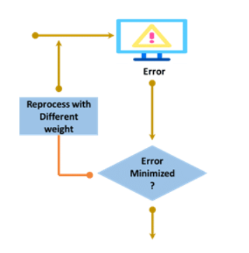
Define errors
what are types of Neural Network
what is the advantage of back propogation over forward propogation

What is an Artificial Neural Network?
A Neural Network is a system designed to operate like a human brain. Human information processing takes place through the interaction of many billions of neurons connected to each other sending signals to other neurons.
Similarly, a Neural Network is a network of artificial neurons, as found in human brains, for solving artificial intelligence problems such as image identification. They may be a physical device or mathematical constructs.
In other words, Artificial Neural Network is a parallel computational system consisting of many simple processing elements connected to perform a particular task.

Biological Motivation
In the above topic, you learned about the Neural Network. Now there is a question which you might be wondering that what motivates towards Neural Network?
Motivation behind neural network is human brain. Human brain is called as the best processor even though it works slower than other computers. Many researchers thought to make a machine that would work in the prospective of the human brain.
Human brain contains billion of neurons which are connected to many other neurons to form a network so that if it sees any image, it recognizes the image and processes the output.

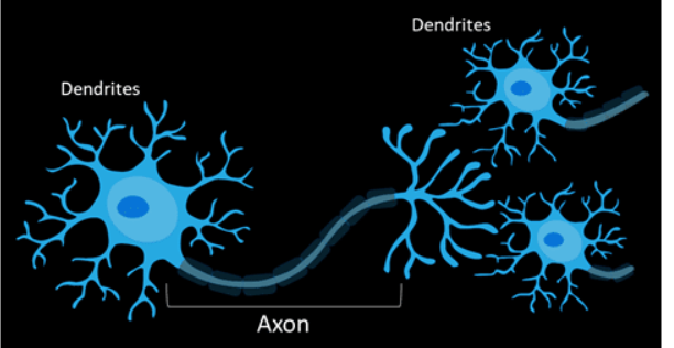
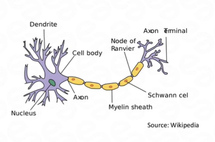
1. Dendrite receives signals from other neurons.
2. Cell body sums the incoming signals to generate input.
3. When the sum reaches a threshold value, neuron fires and the signal travels down the axon to the other neurons.
4. The amount of signal transmitted depend upon the strength of the connections.
5. Connections can be inhibitory, i.e. decreasing strength or excitatory, i.e. increasing strength in nature

.In the similar manner, it was thought to make artificial interconnected neurons like biological neurons making up an Artificial Neural Network(ANN). Each biological neuron is capable of taking a number of inputs and produce output.
Neurons in human brain are capable of making very complex decisions, so this means they run many parallel processes for a particular task. One motivation for ANN is that to work for a particular task identification through many parallel processes

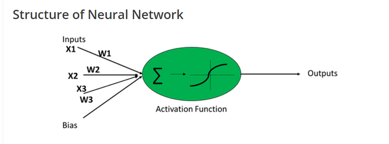
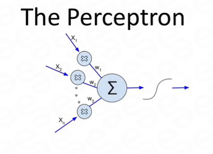
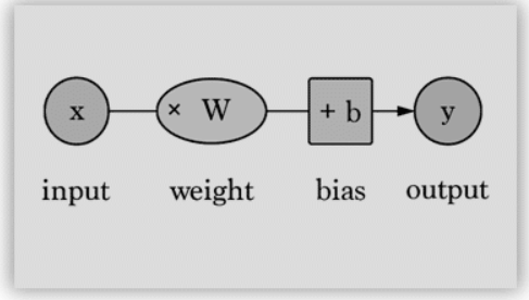
Artificial Neuron
Artificial Neuron are also called as perceptrons. This consist of the following basic terms:

1. Input
2. Weight
3. Bias
4. Activation Function
5. Output How perceptron works? A. All the inputs X1, X2, X3,…., Xn multiplies with their respective weights.

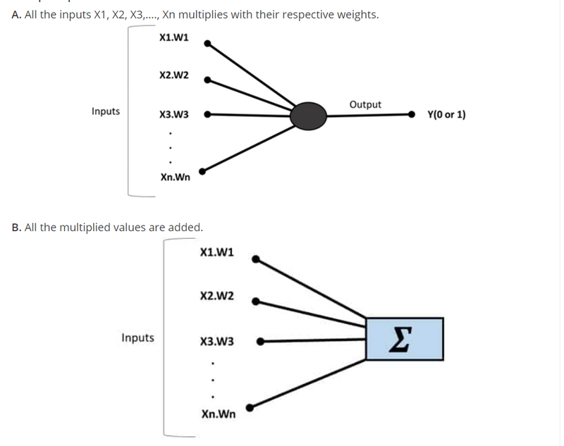
C. Sum of the values are applied to the activation function.

Weights and Bias
Weights W1, W2, W3,…., Wn shows the strength of a neuron.
Bias allows you to change/vary the curve of the activation curve.
Weight without bias curve graph:

W1 = 0.5
W2 = 1.0
W3 = 2.0
X1 = 'w = 0.5'
X2 = 'w = 1.0'
X3 = 'w = 2.0'
for W, X in [(W1, X1), (W2, X2), (W3, X3)]:
f = 1 / (1 + np.exp(-X*W))
plt.plot(X, f, label=l)
plt.xlabel('x')
plt.ylabel('h_w(x)')
plt.legend(loc=2)
plt.show()

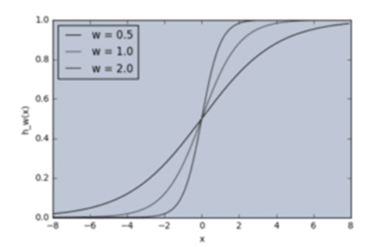
Here, by changing weights, you can very input and outputs. Different weights changes the output slope of the activation function. This can be useful to model Input-Output relationships.
What if you only want output to be changed when X>1? Here, the role of bias starts.
Let’s alter the above example with bias as input.

w = 5.0
b1 = -8.0
b2 = 0.0
b3 = 8.0
X1 = 'b = -8.0'
X2 = 'b = 0.0'
X3 = 'b = 8.0'
for b, X in [(b1,Xl1), (b2, X2), (b3, X3)]:
f = 1 / (1 + np.exp(-(X*w+b)))
plt.plot(X, f, label=l)
plt.xlabel('x')
plt.ylabel('h_wb(x)')
plt.legend(loc=2)
plt.show()

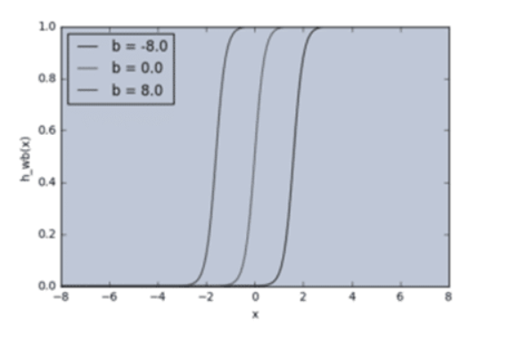
As you can see, by varying the bias b, you can change when the node activates. Without a bias, you cannot vary the output.

Input layer, Hidden layer and Output layer

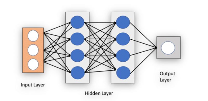
Input Layer
Input layer contains inputs and weights. Example: X1, W1, etc.
Hidden Layer
In a neural network, there can be more than one hidden layer. Hidden layer contains the summation and activation function.
Output Layer
Output layer consists the set of results generated by the previous layer. It also contains the desired value, i.e. values that are already present in the output layer to check with the values generated by the previous layer. It may be also used to improve the end results.
Let’s understand with an example.
Suppose you want to go to a food shop. Based on the three factors you will decide whether to go out or not, i.e.

1. Weather is good or not, i.e. X1. Say X1=1 for good weather and X1=0 for bad weather.
2. You have vehicle available or not, i.e. X2. Say X2=1 for vehicle available and X2=0 for not having vehicle.
3. You have money or not, i.e. X3. Say X3=1 for having money and X3=0 for not having money . Based on the conditions, you choose weight on each condition like W1=6 for money as money is the first important thing you must have, W2=2 for vehicle and W3=2 for weather and say you have set threshold to 5. In this way, perceptron makes decision making model by calculating X1W1, X2W2, and X3W3 and comparing these values to the desired output.

Activation Function
Activation functions are used for non-linear complex functional mappings between the inputs and required variable. They introduce non-linear properties to our Network.
They convert an input of an artificial neuron to output. That output signal now is used as input in the next layer.

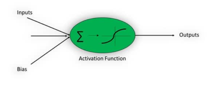
Simply, input between the required values like (0, 1) or (-1, 1) are mapped with the activation function.
Why Activation Function?
Activation Function helps to solve the complex non-linear model. Without activation function, output signal will just be a linear function and your neural network will not be able to learn complex data such as audio, image, speech, etc.
Some commonly used activation functions are:

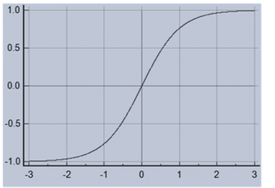
1. Sigmoid or Logistic
2. Tanh — Hyperbolic tangent
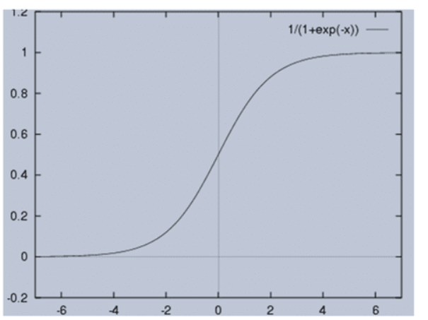
3. ReLu -Rectified linear units Sigmoid Activation Function:

Sigmoid Activation Function can be represented as:

f(x) = 1 / 1 + exp(-x)

1. Rangeof sigmoid function is between 0 and 1.
2. It has some disadvantages like slow convergence, vanishing gradient problem or it kill gradient, etc. Output of Sigmoid is not zero centered that makes its gradient to go in different directions . Tanh- Hyperbolic tangent

Tanh can be represented as:

f(x) = 1 — exp(-2x) / 1 + exp(-2x)

It solves the problem occurring with Sigmoid function. Output of Tanh is zero centered because rangeis between -1 and 1.
Optimization is easy as compared to Sigmoid function.

But still it suffers gradient vanishing problem.
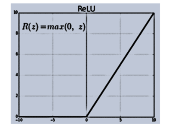
ReLu- Rectified Linear units

It can be represented as:

 R(x) = max(0,x)
 if x < 0 , R(x) = 0 and if x >= 0 , R(x) = x

It avoids as well as rectifies vanishing gradient problem. It has six times better convergence as compared to tanh function.

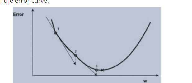
Gradient Descent
Gradient is the slope of the error curve.

Gradient Descent
The idea of introducing gradient to reduce the or minimize the error between the desired output and the input. To predict the output based on the every input, weight must be varied to minimize the error.
Problem is how to vary weight seeing the output error. This can be solved by gradient descent.
In the above graph, blue plot shows the error, red dot shows the ‘w’ value to minimize the error and the black cross or line show the gradient.
At point 1, random ‘w’ value is selected with respect to error and gradient is checked.
If gradient is positive with respect to the increase in w, then step towards will increase the error and if it is negative with respect to increase in ‘w’, then step towards will decrease the error. In this way, gradient shows the direction of the error curve.
The process of minimizing error will continue till the output value reaches close to the desired output. This is a type of Backpropagation.
Wnew=Wold–α ∗∇error
Wnew= new ‘w’ position
Wold= current or old ‘w’ position
∇error= gradient of error at Wold.
α= how quickly converges to minimum error
Example:

Minimum value of the equation f(x)=x4–3x3+2

Minimum value of x is 2.25 by mathematical calculation, so program must give the gradient for that.

x_old = 0
x_new = 6
gamma = 0.01 # step size
precision = 0.00001
def df(x):
y = 4 * x**3 - 9 * x**2
return y

Output:

2.249965

Become a Data Science Architect IBM

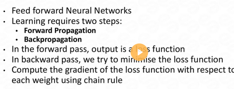
Feed-Forward Neural Network
Feed-forward network means data flows in only one direction, i.e. from input to output.
In gradient topic, you have studied about minimizing the error. The main agenda is also to minimize the error and for that there are various methods.
In feed-forward neural network, when the input is given to the network before going to the next process, it guesses the output by judging the input value. After guess, it checks the guessing value to the desired output value. The difference between the guessing value and the desired output is error.

Guess= input * weight
Error= Desired Output – Guess

You already know how to minimize the error.

Check out this Advanced Computer Vision and Deep Learning course to enhance your Knowledge!

Single Layer Perceptron and Problem with Single Layer Perceptron
Single Layer Perceptron is a linear classifier and if the cases are not linearly separable the learning process will never reach a point where all cases are classified properly.
It is a type of form feed neural network and works like a regular Neural Network.
Example:

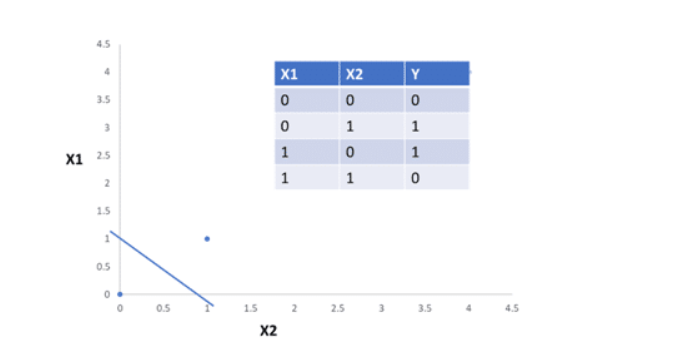
In the above picture, you can see that it is impossible to draw a straight line in case of XOR. So, linear classifier fails in case of Single Layer Perceptron.

Become Master of Machine Learning by going through this online Machine Learning course in Singapore.

Multi-Layer Perceptron(MLP)
It is a type of feed-forward network.
This propagation uses backpropagation.
However, multilayer perceptron uses the backpropagation algorithm that can successfully classify the XOR data.

A multilayer perceptron (MLP) has the same structure as that of the single layer perceptron with one or more hidden layers.
It uses a non-linear activation function and utilizes backpropagation for training. For example, speech recognition and machine translation.
Multi-Layer Perceptron(MLP)
This is how backpropagation works. It uses gradient descent algorithm.
Let’s see a program that explains the multi-layer propagation

//assume all the necessary package classes are imported

public class XorMLP{
public static void main(String[] args) {
// XOR function
DataSettrainingSet = new DataSet(2, 1);
trainingSet.addRow(new DataSetRow(new double[]{0, 0}, new double[]{0}));
trainingSet.addRow(new DataSetRow(new double[]{0, 1}, new double[]{1}));
trainingSet.addRow(new DataSetRow(new double[]{1, 0}, new double[]{1}));
trainingSet.addRow(new DataSetRow(new double[]{1, 1}, new double[]{0}));
// MLP
MultiLayerPerceptronML = newMultiLayerPerceptron(TransferFunctionType.TANH, 2, 3, 1);
// learn the training set
ML.learn(trainingSet);
// test perceptron
System.out.println("Testing trained neural network");
testNeuralNetwork(ML, trainingSet);
// save NN
ML.save("ML.nnet");
// load NN
NeuralNetworkloadML = NeuralNetwork.createFromFile("ML.nnet");
// test NN
System.out.println("Testing loaded neural network");
testNeuralNetwork(loadML, trainingSet);
}
public static void testNeuralNetwork(NeuralNetworknn, DataSettestSet){
for(DataSetRowdataRow : testSet.getRows()) {
nn.setInput(dataRow.getInput());
nn.calculate();
double[ ] Output = nn.getOutput();
System.out.print("Input: " + Arrays.toString(dataRow.getInput()) );
System.out.println(" Output: " + Arrays.toString(Output) );
}
}
}

Run the above code and you will get the main output as 0.862 which is close to the desired output 1. Small error is acceptable.

Types of Neural Network

Mainly used Neural networks are:
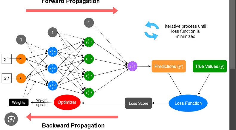
Forward propagation and backpropagation are key concepts in feedforward neural networks, which are the most common type of artificial neural networks. Let's explain these concepts with the help of image examples:

Forward Propagation:
Forward propagation refers to the process of passing input data through the neural network in the forward direction, from the input layer to the output layer. Each neuron in a layer receives inputs from the previous layer, performs a linear combination of the inputs, applies an activation function, and passes the output to the next layer.
Here's an example to illustrate forward propagation:

Forward Propagation

In the image, we have a simple feedforward neural network with one input layer, one hidden layer, and one output layer. The input layer has three input neurons, the hidden layer has four neurons, and the output layer has two neurons.

During forward propagation, the inputs are multiplied by the corresponding weights and passed through activation functions to generate the outputs. The outputs from the previous layer become the inputs for the next layer, and this process continues until the final outputs are generated.

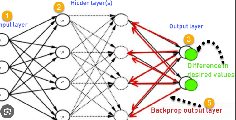
Backpropagation:
Backpropagation, short for "backward propagation of errors," is the process of updating the weights of the neural network by propagating the errors backward from the output layer to the input layer. It calculates the gradient of the loss function with respect to each weight in the network and adjusts the weights accordingly to minimize the error.
Here's an example to illustrate backpropagation:

Backpropagation

In this image, we have the same neural network as before. After the forward propagation step, we compare the predicted outputs with the target outputs and calculate the loss. Backpropagation calculates the gradient of the loss with respect to each weight in the network using the chain rule of derivatives.

The calculated gradients are then used to update the weights in the network. This process is repeated for each training example in the dataset, and the weights are iteratively adjusted to minimize the loss and improve the network's performance.

By iteratively performing forward propagation and backpropagation on a training dataset, a feedforward neural network learns to make accurate predictions by adjusting its weights to minimize the difference between predicted and target outputs.

Convolutional Neural Network(CNN)
Recursive Neural Network(RNN)
Recurrent neural network (RNN)
Long short-term memory (LSTM)
Convolutional Neural Network(CNN)/ ConvNets

Images having high pixels cannot be checked under MLP or regular neural network. In CIFAR-10, images are of the size 32*32*3., i.e. 3072 weights. But for image with size 200*200*3, i.e. 120,000 weights, number of neurons required will be more. So, fully connectivity is not so useful in this situation.
In CNN, the input consists of images and the layers having neurons in three-dimensional structure, i.e. width, height, depth.
Example:
In CIFAR-10, the input volume has dimensions, i.e. width, height, depth 32*32*3.
Convolutional Neural Network(CNN)
In convolutional layer, neurons receive input from only a restricted subarea of the previous layer, i.e. neurons will be only connected to a small region to the layer before it and not in the fully connecting manners.
So, the output layer for CIFAR-10 would have dimensions 1*1*10 because by the end of the CNN the full image will get converted into a small vector along its depth.
A simple CNN for CIFAR-10 has the following sections:

Input(32*32*3), i.e. width 32, height 32 and 3 colour channels red, blue and green.
Convolution layer connects the output of the neurons. This will result in the volume 32*32*8 if you decided to use 8 filters.
Activation Function( ReLu) will apply an activation function that leaves the volume as it is.
Pooling layer will perform down-sampling that reduces the volume to 16*16*8.

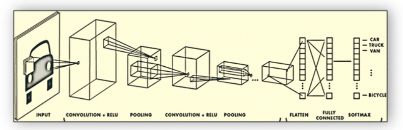
Fully connected layer computes the class score resulting in 1*1*10 volume. Each neuron will be connected to the previous layer numbers just like the regular neural network.
In this way, CNN transforms the image layer by layer to the class score.
It is not important that all the layers contain the same parameters.
CNN transforms
CNN Overview:

Input volume(W1, H1, D1)
Parameters K for number of filters, receptive field size F, stride S and zero padding P.
S is used to mention numbers so that how to slide filters can be known. Example, S=2 means slide the filter by 2. This helps to reduce the volume.
P is used to pad the input borders by 0. It helps to control the size of the output volume.
Output produced having volume W2, H2, D2 where
W2= (W1-F+2P)/S+1
H2=(H1-F+2P)/S+1
D2=K

Parameter sharing, i.e. used to control the parameters. This helps in reusing the parameters. It introduces F.F.D1 weights per filter for total of (F.F.D1).K weights and K bias.

Recursive Neural Network(RNN)
You have learned how to represent a single word. But how could you represent phrases or sentences?
Also, can you model relation between words and multi-word expressions?
Example: “consider” = “take into account” or can you extract representations of full sentences that preserve some of its semantic meaning?
Example: “words representation learned from Intellipaat” = “Intellipaat trained you on text data sets representations”
To solve this problem recursive neural network was introduced.
It uses binary tree and is trained to identify related phrases or sentences.
Example: A wise person suddenly enters the Intellipaat
Recursive Neural Network(RNN)

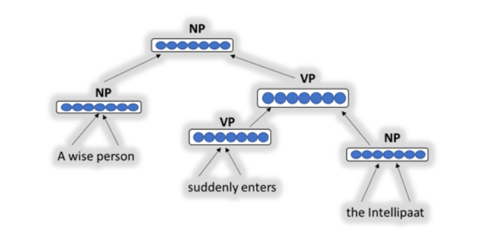
The idea of recursive neural network is to recursively merge pairs of a representation of smaller segments to get representations uncover bigger segments.
The tree structure works on the two following rules:

The semantic representation if the two nodes are merged.
Score of how plausible the new node would be, i.e. how matching the two merged words are.
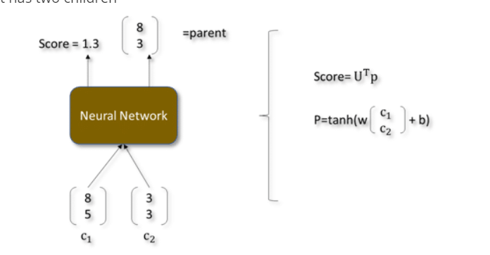
Let’s say a parent has two children
semantic representation
In place of and , there can be two words from a sentence as seen in the above picture. By checking the scores of each pair it produces the output.

What is RNN?

Recursive neural networks architecture can operate on structured input without time limiting to the input sequences. RNN uses parse-tree structural representations.
RNN are also called deep neural network. RNN have been successful in natural language processing(mainly phrases and sentences).
This helps to solve connected handwriting related problems or speech recognition.
Recurrent neural network (RNN)
Recurrent NN is a simplified version of Recursive NN where the time factor is the main factor between the input elements.
Recurrent neural network (RNN)

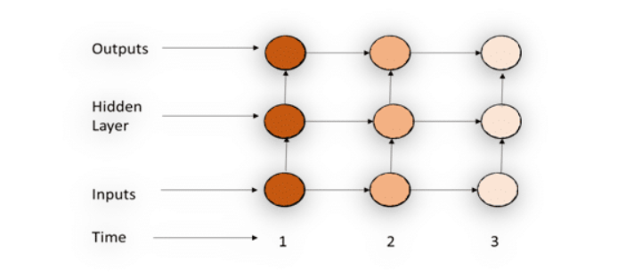
In the above picture, at each time step, in addition to the user’s input, it also accepts the output of the previous hidden layer. Recurrent NN operates on linear chain.
So, you can say that Recursive NN operates on hierarchical structure whereas Recurrent NN operates on the chain structures.
Let’s see what is Recurrent NN:

In Recurrent NN, the information cycles through a loop, i.e. it takes the current input and also what it has learned from the previous layer outputs as shown in the above picture for decision making.
Let’s say you have a normal neural network to which input is Intellipaat. It processes the word character by character. By the time it reaches to the character ‘e’, it has already forgotten about ‘I’, ‘n’, and ‘t’. So, it is impossible for normal neural network to predict next letter.
Recurrent NN remembers that because it has its own internal memory. It produces output, copies that output and loops it back into the network.
Let’s take a practical example to understand Recurrent NN:
Let’s say you are the perfect person for Intellipaat, but why? Because every week, you attain regular courses from Intellipaat to develop your skills. Your schedules are:
Monday = Java, Tuesday = Data Science, Wednesday = Hadoop, Thursday= AWS
develop your skills
If you want a NN to tell you about your next day course then, you have to enter today’s course. So, if you enter input Java then, it should output Data Science. When input is Data Science, then output should be Hadoop, and so on.
Recurrent NN
From the above example, output is recursively is going to the input to judge the next output.

Long short-term memory (LSTM)
What will happen if there are 100 or more than 100 cases in Recurrent NN? What if there are 150 days in a week and you want NN to tell you next day’s course information?
Long short-term memory

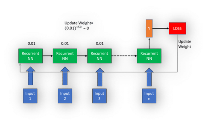
In the above picture, you have 150 states. Each state has a gradient of 0.01. To update the gradient in the first state it would be which is almost equals to zero. So, the update in the weight will become zero. In this case, NN will not learn anything to improve and will produce the same error. This is also called as vanishing gradient problem. This is where LSTM(Long-short term Memory) came into action.
What is LSTM?
Long Short-Term Memory (LSTM) networks are the better version of Recurrent NN that extends Recurrent NN’s memory. LSTM’s memory is like computer’s memory because it can read, write and delete data.
In LSTN there are three gates: input gate, forget gate and output gate. Input gate decides whether to let the input pass or not, forget gate deletes the garbage information and output gate outputs the data at the given time step.
By providing cell gates mechanism to Recurrent NN, LTSM becomes more efficient than Recurrent NN.

Applications of Neural Network

As you are now aware of Neural Network, it’s working and types then, let’s know where it can be implemented.
Neural networks consist of multiple layers that are interconnected to process and transform input data. Each layer performs specific operations and contributes to the overall functionality of the network. Let's explore some commonly used layers in neural networks:

Input Layer:
The input layer is the initial layer that receives the input data. It does not perform any computation and simply passes the input values to the next layer. The number of neurons in the input layer is determined by the number of input features in the dataset.

Dense Layer (Fully Connected Layer):
A dense layer, also known as a fully connected layer, connects each neuron in the current layer to every neuron in the subsequent layer. This layer performs a linear combination of the input values followed by an activation function. It learns weights associated with each connection during training.

Example:

model.add(keras.layers.Dense(units=64, activation='relu'))

In this example, a dense layer with 64 neurons is added to the neural network model. The activation function 'relu' is used, which applies the rectified linear unit activation function element-wise to the output of the layer.

Convolutional Layer:
Convolutional layers are commonly used in convolutional neural networks (CNNs) for image processing tasks. These layers apply a set of learnable filters (kernels) to extract local patterns and features from the input data. Convolutional layers preserve spatial relationships within the input.

Example:

model.add(keras.layers.Conv2D(filters=32, kernel_size=(3, 3), activation='relu'))

In this example, a convolutional layer with 32 filters, each of size 3x3, is added to the model. The activation function 'relu' is applied to the output of the layer.

Pooling Layer:
Pooling layers are often used after convolutional layers in CNNs to reduce the spatial dimensions of the feature maps. They summarize the information in a neighborhood of the input and provide a compact representation. Max pooling and average pooling are common pooling techniques.

Example:

model.add(keras.layers.MaxPooling2D(pool_size=(2, 2)))

In this example, a max pooling layer with a pool size of 2x2 is added to the model. It reduces the spatial dimensions of the input by taking the maximum value within each 2x2 region.

Recurrent Layer:
Recurrent layers are used in recurrent neural networks (RNNs) to handle sequential or time-series data. These layers maintain hidden states and process input sequences iteratively, allowing the network to capture temporal dependencies.

Example:

model.add(keras.layers.LSTM(units=64, activation='tanh'))

Here, an LSTM (Long Short-Term Memory) layer with 64 units is added to the model. LSTM is a type of recurrent layer that can capture long-term dependencies in sequential data.

Output Layer:
The output layer is the final layer in the neural network that produces the desired output or prediction. The number of neurons in the output layer depends on the problem type (e.g., binary classification, multi-class classification, regression).

Example:

model.add(keras.layers.Dense(units=1, activation='sigmoid'))

In this example, an output layer with a single neuron is added to the model. The activation function 'sigmoid' is used to squash the output into the range [0, 1] for binary classification.

Image Recognition/Compression
Character Recognition
Stock Market Prediction
Human Face Recognition
Signature Verification Application
Speech Recognition
Voice Recognition
Character Recognition

machine-learning-tutorial/neural-network-tutorial

A neural network is a computational model inspired by the structure and functioning of biological neural networks in the human brain. It consists of interconnected nodes called neurons, organized in layers. Neural networks are widely used in various machine learning tasks, including classification, regression, and pattern recognition.

Let's explain a basic neural network example for binary classification:

Example:
Suppose we have a dataset with two features (x1, x2) and two classes, "Class A" and "Class B". We want to train a neural network to classify new data points into one of these two classes.

Import the required libraries and create the neural network model:

import numpy as np
from tensorflow import keras

# Create a sequential neural network model
model = keras.Sequential()
Add layers to the neural network:

# Add input layer with 2 input neurons
model.add(keras.layers.Dense(2, input_dim=2, activation='relu'))

# Add output layer with 1 output neuron
model.add(keras.layers.Dense(1, activation='sigmoid'))

In this example, we create a sequential neural network model using the Keras API, which is a high-level neural networks API. We add layers to the model using the add() method. The Dense layer represents a fully connected layer in the neural network. The first layer added is the input layer with 2 input neurons, and the second layer is the output layer with 1 output neuron. The activation functions used are 'relu' for the hidden layer and 'sigmoid' for the output layer.

Compile and train the neural network model:

# Compile the model
model.compile(optimizer='adam', loss='binary_crossentropy', metrics=['accuracy'])

# Prepare the training data and labels
X_train = np.array([(1, 2), (2, 3), (3, 3), (6, 5), (7, 7), (8, 6)])
y_train = np.array([0, 0, 0, 1, 1, 1])

Train the model

model.fit(X_train, y_train, epochs=100, batch_size=2)

Here, we compile the model by specifying the optimizer, loss function, and metrics to be used during training. We then prepare the training data and labels as numpy arrays. Finally, we train the model using the fit() method, specifying the number of epochs (iterations over the training data) and the batch size.

Make predictions on new data points:

# Prepare new data points for prediction
X_new = np.array([(4, 4), (1, 1)])

# Predict the classes for the new data points
y_pred = model.predict(X_new)

print(y_pred)

We can use the trained model to make predictions on new data points using the predict() method. In this example, we provide the new data points (X_new) to the model, and it returns the predicted class probabilities for each data point.

Output:
The output of the code snippet will be the predicted class probabilities for the new data points. Since it is a binary classification task, the output will be a probability value between 0 and 1.

For example:

[[0.742]
 [0.254]]

The output indicates the predicted probabilities of the data points belonging to the positive class (Class B). The first data point has a probability of 0.742 of belonging to Class B, and the second data point has a probability of 0.254 of belonging to Class B.

why we add bias

Adjusting Activation Threshold: Bias allows the activation threshold of the neuron to be adjusted. Without bias, the neuron would always activate only when the input is zero, which limits the flexibility of the model. With bias, the neuron can activate even when the input is not zero.

Enabling Shift of Activation Function: Bias helps in shifting the activation function to the left or right, making it possible for the model to learn and approximate more complex functions.

Improving Model Flexibility: Bias terms provide additional degrees of freedom, making the model more capable of fitting the data by learning the optimal parameters.

Handling Data Distribution: In real-world data, features often do not have a mean of zero. Bias helps in adjusting the model to better fit such data distributions.

Preventing Dead Neurons: In neural networks with activation functions like ReLU, without bias, there's a higher chance of neurons becoming inactive (dead neurons). Bias helps in preventing this by ensuring that neurons can still activate even with negative or zero input.