why we use computational graph
How computational graph play fundamental role in creating and training machine learning models
Basic Operation of computational graph in tensor flow
why we use computational graph
In TensorFlow, a computation is represented as a directed acyclic graph (DAG) of operations. Each node in the graph represents an operation, and the edges define the flow of tensors between operations. Here's a checklist of common graph operations in TensorFlow along with examples:
Computation graph
In TensorFlow, a computational graph is a way to represent a mathematical computation as a directed graph, where nodes in the graph represent mathematical operations, and edges represent the flow of data between these operations. This graph-based representation allows TensorFlow to optimize the execution of computations, distribute them across multiple devices, and efficiently compute gradients for optimization algorithms like backpropagation.
The computational graph, represents the structure of the neural network or model, and TensorFlow's session execution is used to perform the actual computations on this graph. The graph allows TensorFlow to efficiently optimize and parallelize the computations, and it provides a foundation for implementing automatic differentiation during backpropagation for training the model.
Here are a few reasons why computational graphs are used in TensorFlow:
Graph Optimization: TensorFlow can optimize the computational graph before execution. Common subexpressions can be identified and computed only once, and unnecessary operations can be eliminated. This optimization can lead to faster execution of the overall computation.
Parallelism: TensorFlow can automatically distribute computations across multiple devices (such as GPUs) or machines. The graph structure helps in identifying independent subgraphs that can be executed in parallel, leading to improved performance.
Automatic Differentiation: TensorFlow can automatically compute gradients for variables in the computational graph using automatic differentiation. This is crucial for training machine learning models using optimization algorithms like gradient descent. The graph structure makes it easier to compute gradients using backpropagation.
Here's a simple example to illustrate the concept of a computational graph in TensorFlow:
import tensorflow as tf
# Define input placeholders
x = tf.placeholder(tf.float32, name='x')
y = tf.placeholder(tf.float32, name='y')
# Define operations in the graph
add_op = tf.add(x, y, name='addition')
multiply_op = tf.multiply(add_op, 2, name='multiplication')
# Create a session to execute the graph
with tf.Session() as sess:
# Define input values
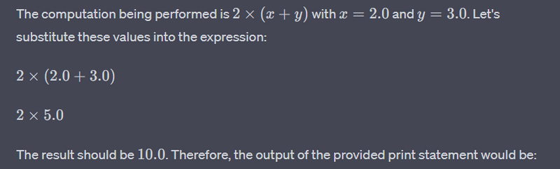
x_value = 2.0
y_value = 3.0
# Feed values into the graph and execute
result = sess.run(multiply_op, feed_dict={x: x_value, y: y_value})
# Output the result
print(f"The result of (2 * (x + y)) with x={x_value} and y={y_value} is: {result}")
output
How computational graph play fundamental role in creating and training machine learning models
a computational graph is a fundamental concept in TensorFlow and is integral to the process of creating and training machine learning models. When you define a model in TensorFlow, you are essentially creating a computational graph that represents the mathematical operations involved in the model.
Here's a simplified overview of how a computational graph is used to create a model in TensorFlow:
Define the Model Architecture:
- Define the input placeholders for the model, representing the input data.
- Define the variables, which are the model parameters to be learned during training.
- Specify the operations that define the forward pass of the model, connecting the inputs to the output .
import tensorflow as tf
# Define input placeholder
x = tf.placeholder(tf.float32, shape=[None, input_size], name='input_placeholder')

# Define variables (model parameters)
W = tf.Variable(tf.random_normal([input_size, output_size]), name='weights')
b = tf.Variable(tf.zeros([output_size]), name='bias')

# Define the model's forward pass
output = tf.matmul(x, W) + b
Define the Loss Function:
Define a loss function that measures the difference between the model's predictions and the actual target values.
# Define target placeholder
y_true = tf.placeholder(tf.float32, shape=[None, output_size], name='target_placeholder')

# Define the loss function (e.g., mean squared error)
loss = tf.reduce_mean(tf.square(output - y_true))
Optimization and Training:
Choose an optimization algorithm (e.g., gradient descent) and specify a learning rate.
Define an optimizer to minimize the loss.
# Choose an optimizer and specify a learning rate
optimizer = tf.train.GradientDescentOptimizer(learning_rate=0.01)

# Define the training operation
train_op = optimizer.minimize(loss)
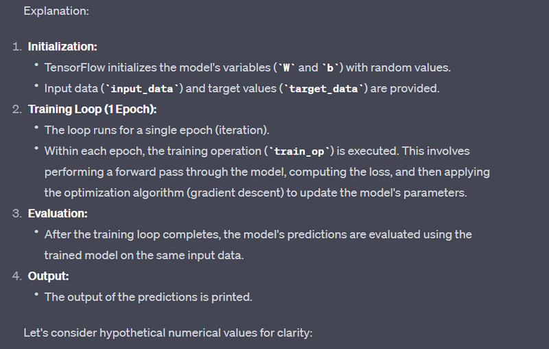
Session Execution:
Create a TensorFlow session.
Initialize variables.
Feed the input data and target values into the graph to train the model.
# For simplicity, let's assume some random input_data and target_data
input_data = [[1.0, 2.0], [2.0, 3.0], [3.0, 4.0]]
target_data = [[3.0], [5.0], [7.0]]

# Assuming num_epochs is set to 1 for simplicity
num_epochs = 1

with tf.Session() as sess:
    # Initialize variables
    sess.run(tf.global_variables_initializer())

    # Training loop
    for epoch in range(num_epochs):
        # Feed input data and target values into the graph
        sess.run(train_op, feed_dict={x: input_data, y_true: target_data})

    # After training, you can evaluate the model's predictions
    predictions = sess.run(output, feed_dict={x: input_data})

    # Output the results
    print("Model's Predictions:")
    print(predictions)
The computational graph, in this case, represents the structure of the neural network or model, and TensorFlow's session execution is used to perform the actual computations on this graph. The graph allows TensorFlow to efficiently optimize and parallelize the computations, and it provides a foundation for implementing automatic differentiation during backpropagation for training the model.
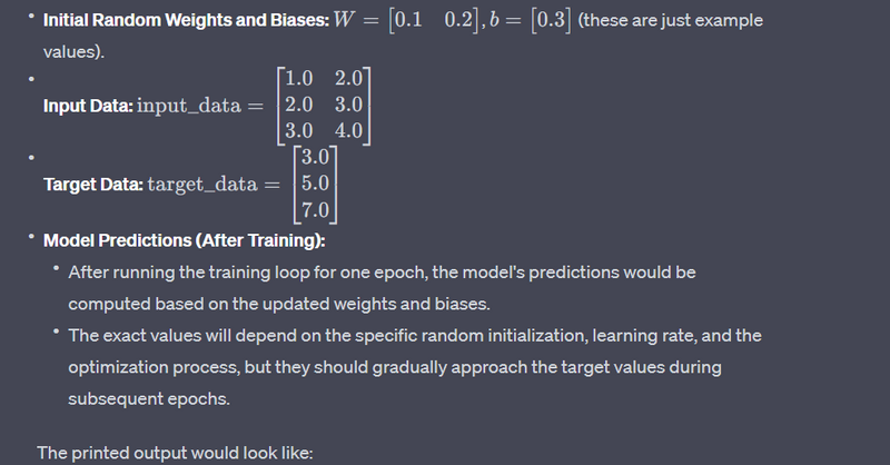
Model's Predictions:
[[0.8708147]
 [1.9320316]
 [2.9932485]]
These are the model's predictions after one epoch of training. In a real-world scenario, you would typically run multiple epochs to allow the model to learn and improve its predictions over time.
A computation graph is the basic unit of computation in TensorFlow. A computation graph consists of nodes and edges. Each node represents an instance of tf.Operation, while each edge represents an instance of tf.Tensor that gets transferred between the nodes.
A model in TensorFlow contains a computation graph. First, you must create the graph with the nodes representing variables, constants, placeholders, and operations, and then provide the graph to the TensorFlow execution engine. The TensorFlow execution engine finds the first set of nodes that it can execute. The execution of these nodes starts the execution of the nodes that follow the sequence of the computation graph.
Thus, TensorFlow-based programs are made up of performing two types of activities on computation graphs:
Defining the computation graph
Executing the computation graph
A TensorFlow program starts execution with a default graph. Unless another graph is explicitly specified, a new node gets implicitly added to the default graph. Explicit access to the default graph can be obtained using the following command:
graph = tf.get_default_graph()
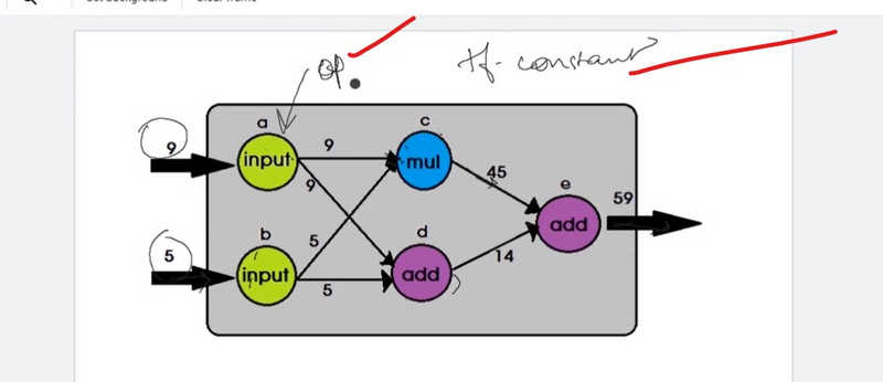
For example, the following computation graph represents the addition of three inputs to produce the output, that is,
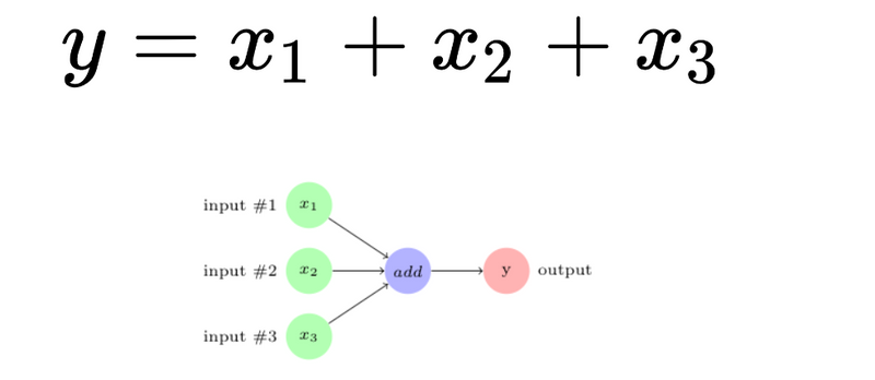
Basic Operation of computational graph in tensor flow
In TensorFlow, the add operation node in the preceding diagram would correspond to the code y = tf.add( x1 + x2 + x3 ).
The variables, constants, and placeholders get added to the graph as and when they are created. After defining the computation graph, a session object is instantiated that executes the operation objects and evaluates the tensor objects.
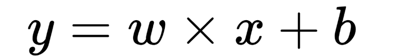
Let's define and execute a computation graph to calculate
, just like we saw in the preceding example:

# Linear Model y = w * x + b
# Define the model parameters
w = tf.Variable([.3], tf.float32)
b = tf.Variable([-.3], tf.float32)
# Define model input and output
x = tf.placeholder(tf.float32)
y = w * x + b
output = 0

with tf.Session() as tfs:
   # initialize and print the variable y
   tf.global_variables_initializer().run()
   output = tfs.run(y,{x:[1,2,3,4]})
print('output : ',output)
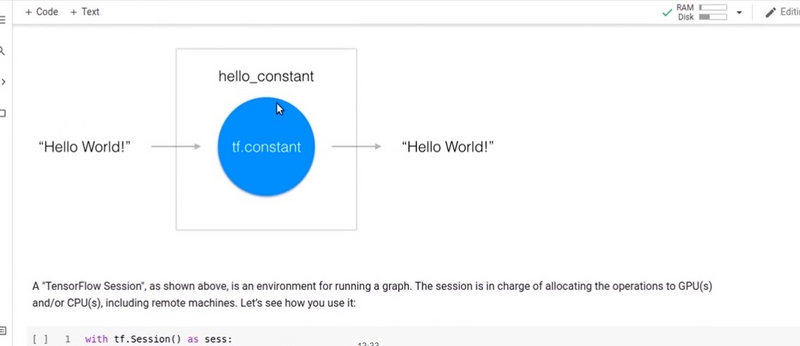
Creating and using a session in the with block ensures that the session is automatically closed when the block is finished. Otherwise, the session has to be explicitly closed with the tfs.close() command, where tfs is the session name.
1. Constants:
Example:
import tensorflow as tf

# Creating a constant tensor
a = tf.constant(5)
b = tf.constant(3)
c = tf.add(a, b)

with tf.compat.v1.Session() as sess:
    result = sess.run(c)
    print(result)  # Output: 8
2. Placeholders:
Example:
import tensorflow as tf

# Creating placeholders
X = tf.compat.v1.placeholder(tf.float32)
Y = X * 2

with tf.compat.v1.Session() as sess:
    result = sess.run(Y, feed_dict={X: 3.5})
    print(result)  # Output: 7.0
3. Variables:
Example:
import tensorflow as tf

# Creating a variable
W = tf.Variable(2.0, name='weight')
b = tf.Variable(1.0, name='bias')

with tf.compat.v1.Session() as sess:
    sess.run(tf.compat.v1.global_variables_initializer())
    print(sess.run([W, b]))  # Output: [2.0, 1.0]
4. Math Operations:
Example:
import tensorflow as tf

# Math operations
a = tf.constant(5)
b = tf.constant(3)
add = tf.add(a, b)
multiply = tf.multiply(a, b)

with tf.compat.v1.Session() as sess:
    result_add, result_multiply = sess.run([add, multiply])
    print(result_add, result_multiply)  # Output: 8, 15
5. Activation Functions:
Example:
import tensorflow as tf

# Activation function (ReLU)
x = tf.constant([-2.0, -1.0, 0.0, 1.0, 2.0])
y = tf.nn.relu(x)

with tf.compat.v1.Session() as sess:
    result = sess.run(y)
    print(result)  # Output: [0. 0. 0. 1. 2.]
6. Matrix Operations:
Example:
import tensorflow as tf

# Matrix multiplication
matrix_a = tf.constant([[2, 3], [4, 5]])
matrix_b = tf.constant([[1, 2], [3, 4]])
product = tf.matmul(matrix_a, matrix_b)

with tf.compat.v1.Session() as sess:
    result = sess.run(product)
    print(result)
    # Output: [[11, 16], [19, 28]]
7. Loss Functions:
Example:
import tensorflow as tf

# Mean Squared Error
predictions = tf.constant([1.0, 2.0, 3.0])
labels = tf.constant([0.0, 2.0, 4.0])
mse = tf.losses.mean_squared_error(labels, predictions)

with tf.compat.v1.Session() as sess:
    result = sess.run(mse)
    print(result)  # Output: 2.0
8. Optimizers:
import tensorflow as tf

# Gradient Descent optimizer
x = tf.Variable(2.0)
y = x**2
optimizer = tf.compat.v1.train.GradientDescentOptimizer(learning_rate=0.1)
train_op = optimizer.minimize(y)

with tf.compat.v1.Session() as sess:
    sess.run(tf.compat.v1.global_variables_initializer())
    for _ in range(100):
        sess.run(train_op)
    result = sess.run(x)
    print(result)  # Output: close to 0.0
9. Neural Network Layers:
import tensorflow as tf

# Dense layer
inputs = tf.constant([[1.0, 2.0, 3.0]])
dense_layer = tf.keras.layers.Dense(units=4, activation='relu')
output = dense_layer(inputs)

with tf.compat.v1.Session() as sess:
    sess.run(tf.compat.v1.global_variables_initializer())
    result = sess.run(output)
    print(result)
[[0. 0. 0. 0.]]
This is because the Dense layer with ReLU activation is applied to the input tensor [[1.0, 2.0, 3.0]], and the output is computed based on the weights and biases of the dense layer. In this case, since the weights are initialized to zero, and ReLU activation sets negative values to zero, the output is [0.0, 0.0, 0.0, 0.0].
If you are using TensorFlow 1.x, the output will be the same, but the way you open and close the session will be slightly different, as shown in the previous response.
10. Session Execution:
import tensorflow as tf

# Creating a session for graph execution
a = tf.constant(5)
b = tf.constant(3)
c = tf.add(a, b)

with tf.compat.v1.Session() as sess:
    result = sess.run(c)
    print(result)  # Output: 8
Note: TensorFlow 2.x encourages eager execution by default, and the tf.compat.v1.Session() is not typically used. The examples above include TensorFlow 1.x-style sessions for demonstration purposes.
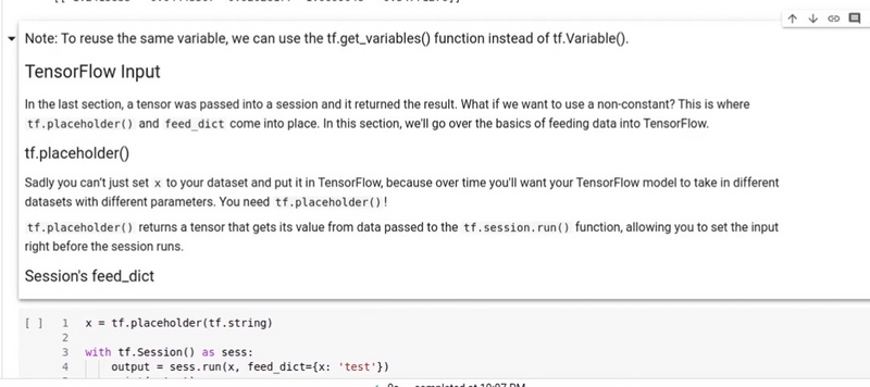
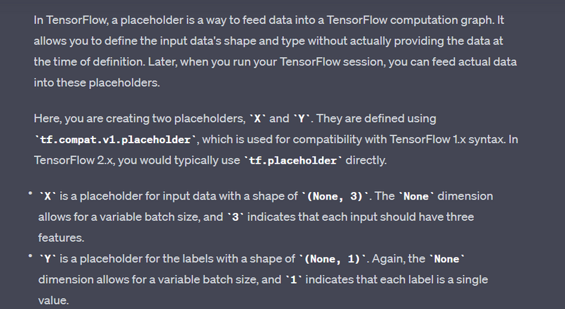
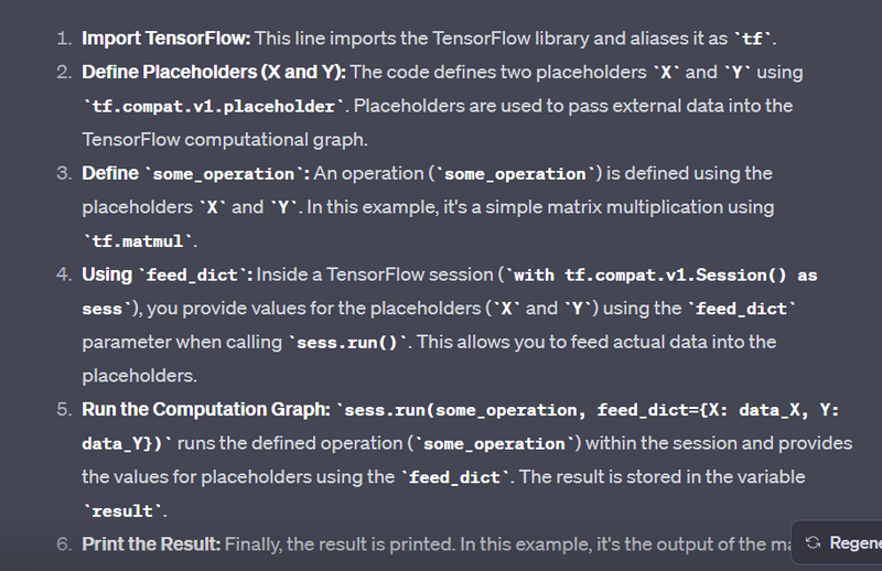
Creating Placeholders:
import tensorflow as tf

# Creating placeholders
X = tf.compat.v1.placeholder(tf.float32, shape=(None, 3))
Y = tf.compat.v1.placeholder(tf.float32, shape=(None, 1))
Explanation
# Example usage in a TensorFlow session
with tf.compat.v1.Session() as sess:
    # Assuming you have some data to feed
    input_data = [[1.0, 2.0, 3.0], [4.0, 5.0, 6.0]]
    labels = [[0.0], [1.0]]

    # Feed the data into the placeholders
    feed_dict = {X: input_data, Y: labels}

    # Now you can perform operations using these placeholders, for example
    result = sess.run(some_operation, feed_dict=feed_dict)
    print(result)
Feed Data using feed_dict
import tensorflow as tf

# Using placeholders with feed_dict
with tf.compat.v1.Session() as sess:
    data_X = [[1.0, 2.0, 3.0], [4.0, 5.0, 6.0]]
    data_Y = [[7.0], [8.0]]

    result = sess.run(some_operation, feed_dict={X: data_X, Y: data_Y})
import tensorflow as tf

# Define placeholders
X = tf.compat.v1.placeholder(tf.float32, shape=(None, 3))
Y = tf.compat.v1.placeholder(tf.float32, shape=(None, 1))

# Define some_operation using X and Y
some_operation = tf.matmul(X, tf.constant([[1.0], [2.0], [3.0]]))

# Using placeholders with feed_dict
with tf.compat.v1.Session() as sess:
    data_X = [[1.0, 2.0, 3.0], [4.0, 5.0, 6.0]]
    data_Y = [[7.0], [8.0]]

    # Run the computation graph and feed data using feed_dict
    result = sess.run(some_operation, feed_dict={X: data_X, Y: data_Y})

# Print the result
print(result)
Another Example
import tensorflow as tf

# Define placeholders
X = tf.compat.v1.placeholder(tf.float32, shape=(None, 3))
Y = tf.compat.v1.placeholder(tf.float32, shape=(None, 1))

# Define a meaningful operation
some_operation = X + tf.constant([[10.0]])

# Using placeholders with feed_dict
with tf.compat.v1.Session() as sess:
    data_X = [[1.0, 2.0, 3.0], [4.0, 5.0, 6.0]]
    data_Y = [[7.0], [8.0]]

    # Run the computation graph and feed data using feed_dict
    result = sess.run(some_operation, feed_dict={X: data_X, Y: data_Y})

# Print the result
print(result)
output
In this example, the operation is a simple addition of the input data X with a constant value 10.0. The output will be the sum of each element in X with 10.0.
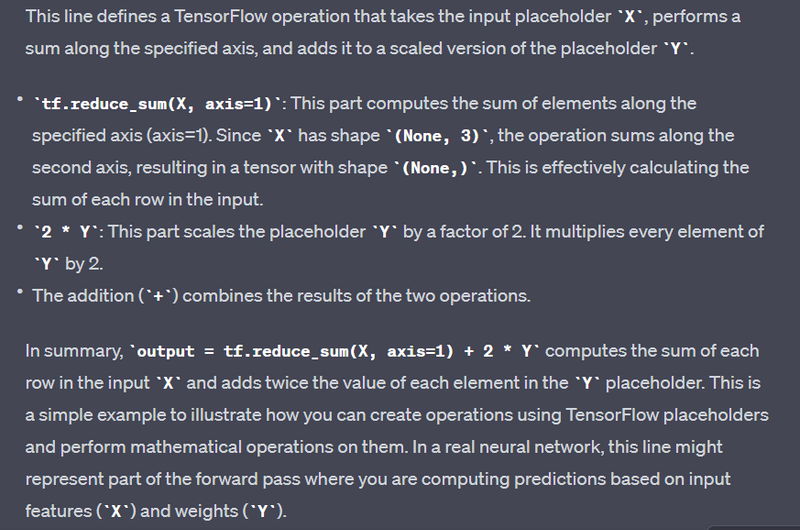
Dynamic Shapes with None:
import tensorflow as tf
import numpy as np
# Using None for dynamic shapes
X = tf.compat.v1.placeholder(tf.float32, shape=(None, 3))
Y = tf.compat.v1.placeholder(tf.float32, shape=(None, 1))
# Some operation (for demonstration purposes)
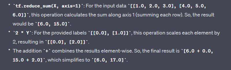
output = tf.reduce_sum(X, axis=1) + 2 * Y
# Example usage in a TensorFlow session
with tf.compat.v1.Session() as sess:
# Assuming you have some data to feed
input_data = np.array([[1.0, 2.0, 3.0], [4.0, 5.0, 6.0]])
labels = np.array([[0.0], [1.0]])
# Feed the data into the placeholders
feed_dict = {X: input_data, Y: labels}
# Run the operation within the session
result = sess.run(output, feed_dict=feed_dict)
print("Input Data:")
print(input_data)
print("Labels:")
print(labels)
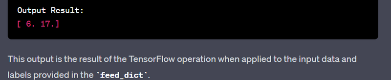
print("Output Result:")
print(result)
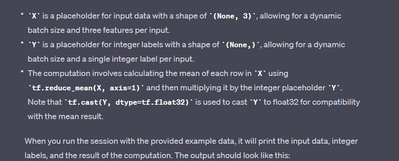
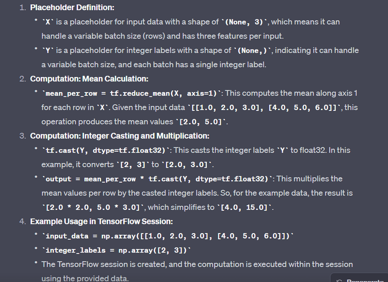
Multiple Placeholder Types:
import tensorflow as tf
import numpy as np

# Using different types of placeholders
X = tf.compat.v1.placeholder(tf.float32, shape=(None, 3))
Y = tf.compat.v1.placeholder(tf.int32, shape=(None,))

# Computation: Mean of each row in X multiplied by Y
mean_per_row = tf.reduce_mean(X, axis=1)
output = mean_per_row * tf.cast(Y, dtype=tf.float32)  # Casting Y to float32 for compatibility

# Example usage in a TensorFlow session
with tf.compat.v1.Session() as sess:
    # Assuming you have some data to feed
    input_data = np.array([[1.0, 2.0, 3.0], [4.0, 5.0, 6.0]])
    integer_labels = np.array([2, 3])

    # Feed the data into the placeholders
    feed_dict = {X: input_data, Y: integer_labels}

    # Run the operation within the session
    result = sess.run(output, feed_dict=feed_dict)

    print("Input Data:")
    print(input_data)
    print("Integer Labels:")
    print(integer_labels)
    print("Output Result:")
    print(result)
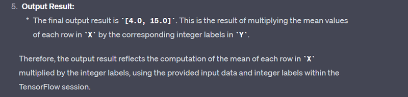
Input Data:
[[1. 2. 3.]
 [4. 5. 6.]]
Integer Labels:
[2 3]
Output Result:
[ 4. 15.]
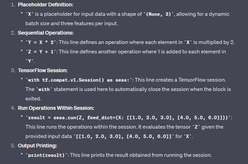
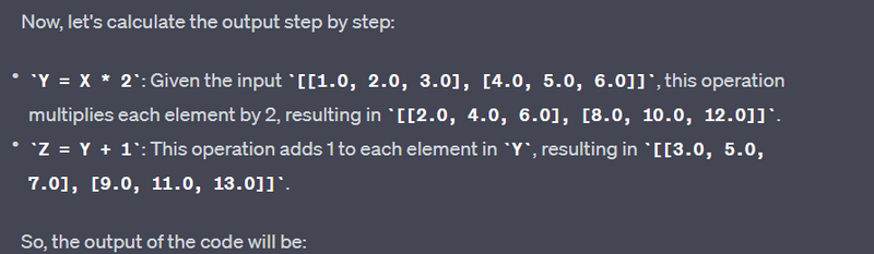
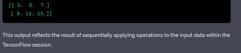
Sequential Operations with Placeholders:
import tensorflow as tf

# Sequential operations with placeholders
X = tf.compat.v1.placeholder(tf.float32, shape=(None, 3))
Y = X * 2
Z = Y + 1

with tf.compat.v1.Session() as sess:
    result = sess.run(Z, feed_dict={X: [[1.0, 2.0, 3.0], [4.0, 5.0, 6.0]]})
    print(result)
Batch Processing:

Top comments (0)