when decision tree algorithm is used in ml
Explain tree prunning and when it is to be used
How decision tree constructed and split based on entropy and gini impurity
Decision Tree Algorithm:
The Decision Tree algorithm is a supervised learning algorithm used for both classification and regression tasks. It builds a tree-like model by recursively splitting the dataset based on the values of different features. Each internal node of the tree represents a feature, each branch represents a decision rule, and each leaf node represents a class label or a predicted value.
Example:
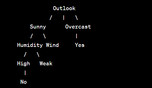
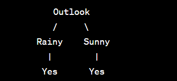
Let's consider a binary classification problem to predict whether a person will play tennis based on weather conditions. We have a dataset with the following features: Outlook, Temperature, Humidity, and Wind, and the corresponding labels: PlayTennis (Yes or No).
Outlook Temperature Humidity Wind PlayTennis
Sunny Hot High Weak No
Sunny Hot High Strong No
Overcast Hot High Weak Yes
Rainy Mild High Weak Yes
Rainy Cool Normal Weak Yes
Overcast Cool Normal Strong Yes
Sunny Mild High Weak No
Sunny Cool Normal Weak Yes
Rainy Mild Normal Weak Yes
Sunny Mild Normal Strong Yes
Overcast Mild High Strong Yes
Overcast Hot Normal Weak Yes
Rainy Mild High Strong No
Output:
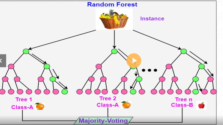
A decision tree generated from this dataset might look like this:
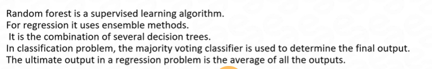
Random Forest Algorithm:
Random Forest is an ensemble learning algorithm that combines multiple decision trees to make predictions. It creates a "forest" of decision trees, each trained on a randomly selected subset of the training data and a subset of features. The final prediction is made by aggregating the predictions of all individual trees through voting (for classification) or averaging (for regression).
Example:
Continuing from the previous example, let's apply the Random Forest algorithm to the tennis dataset.
Output:
A Random Forest model may consist of multiple decision trees, each trained on different subsets of data and features. The following is an example of three decision trees in the Random Forest model:
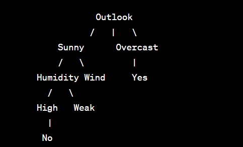
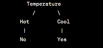
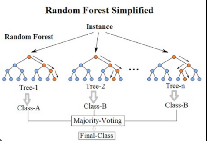
The Random Forest model combines the predictions of these three trees (through voting) to make the final prediction.
Output:
For a new example with the feature values: Outlook = Sunny, Temperature = Cool, Humidity = High, Wind = Strong, the Random Forest model will make predictions using each decision tree and combine the results to determine the final prediction. If two out of three trees predict "Yes" and one predicts "No," the Random Forest may predict "Yes" as the final outcome.
when decision tree algorithm is used in ml
Decision tree algorithms are widely used in machine learning for both classification and regression tasks. They are versatile and powerful algorithms that can handle both categorical and numerical data. Decision trees create a tree-like model of decisions and their potential consequences, making them intuitive and easy to interpret. Here are some common scenarios where decision tree algorithms are used:
Classification Problems:
Decision trees are commonly used for classification tasks, where the goal is to predict the class or category of an input data point. Decision trees work well with categorical features and can handle multi-class classification problems effectively.
Example: Classifying whether an email is spam or not spam based on various features like the presence of certain words, email sender, and email length.
Regression Problems:
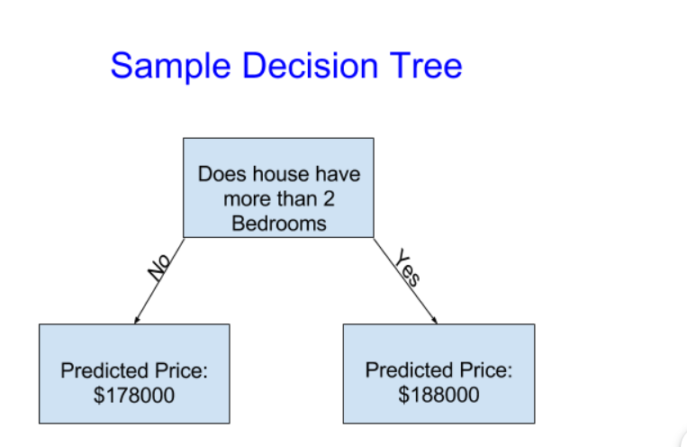
Decision trees can be used for regression tasks, where the goal is to predict a continuous numerical value. They partition the data into regions and predict the average value within each region.
Example: Predicting the price of a house based on features such as the number of bedrooms, square footage, and location.
Ensemble Methods:
Decision trees are often used as base learners in ensemble methods such as Random Forest and Gradient Boosting. Ensemble methods combine multiple decision trees to create more robust and accurate models.
Example: Random Forest combines multiple decision trees to improve the accuracy of the classification or regression tasks.
Feature Importance Analysis:
Decision trees provide a natural way to measure the importance of features in a dataset. By observing which features are used near the root of the tree, we can understand which features have the most significant impact on the target variable.
Example: Identifying the most important features that affect customer churn in a subscription-based service.
Interpretable Models:
Decision trees are one of the most interpretable machine learning models. Their hierarchical structure allows humans to follow the decision-making process step-by-step.
Example: In medical diagnosis, decision trees can be used to explain the rules followed to classify a patient's disease, making it easier for doctors to understand and trust the model's predictions.
Handling Non-Linear Relationships:
Decision trees can model non-linear relationships between features and the target variable. By recursively splitting the data based on different features, they can capture complex patterns.
Example: Predicting a person's income based on age, education level, and work experience, where the relationship between income and these features may not be linear.
While decision trees have many advantages, they can suffer from overfitting when they become too complex. Regularization techniques, ensemble methods, and hyperparameter tuning are used to address this issue and improve the model's generalization performance. Overall, decision trees are valuable tools in the data scientist's toolkit, capable of handling a wide range of machine learning tasks.
Explain tree prunning and when it is to be used
Tree pruning, also known as tree regularization or tree trimming, is a technique used to reduce the complexity of decision trees by removing some branches (nodes) that do not contribute much to the overall predictive power of the tree. Pruning helps prevent overfitting, where the tree memorizes the training data but performs poorly on new, unseen data. By removing unnecessary branches, pruned trees are more generalized and have better performance on unseen data.
Example of Tree Pruning:
Let's consider a simple decision tree for a classification problem that predicts whether a person will buy a product based on two features: age and income.
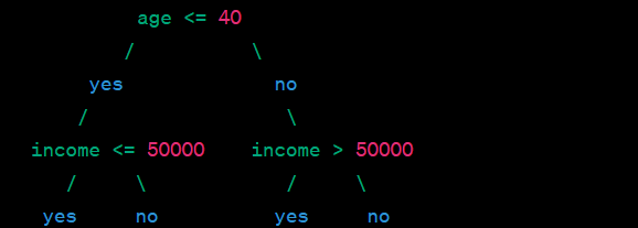
In this example, the tree has four levels (including the root). Each node represents a decision based on a specific feature and its threshold. The leaf nodes represent the final decision (yes or no) for the classification task.
The tree appears to be fitting the training data perfectly. However, we suspect it might be overfitting. To address this issue, we can perform tree pruning.
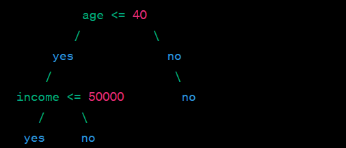
Suppose that during the pruning process, the algorithm identifies that the node "income > 50000" does not add significant predictive power to the tree and may be a result of random fluctuations in the training data. Pruning this node would remove the unnecessary complexity.
After pruning, the tree might look like this:
As a result of pruning, the tree has become simpler, with fewer levels and fewer decision nodes. By removing the unnecessary node "income > 50000," the pruned tree is less likely to overfit the training data and is more likely to generalize well on new, unseen data.
Tree pruning is typically done using algorithms like Reduced Error Pruning, Cost Complexity Pruning (also known as Minimal Cost-Complexity Pruning), or Rule Post-Pruning, depending on the specific pruning strategy and criteria. Pruning is an essential step in building robust decision trees that strike a balance between complexity and accuracy in machine learning tasks.
When tree prunning is used
Tree pruning is used in machine learning to prevent decision trees from overfitting, especially when dealing with complex datasets. Overfitting occurs when a decision tree learns the training data too well, capturing noise and irrelevant patterns, which leads to poor performance on new, unseen data. Pruning helps to address this issue by simplifying the tree and reducing its complexity.
Tree pruning is applied in the following scenarios in machine learning:
Large Decision Trees:
When decision trees grow large and deep, they become more susceptible to overfitting. Pruning is used to cut off branches that do not contribute much to the tree's predictive power, effectively reducing the tree's size.
Complex Datasets:
In complex datasets with noise or irrelevant features, decision trees can easily memorize noise rather than discovering meaningful patterns. Pruning helps remove the noise and focus on relevant patterns.
Reducing Computational Complexity:
Pruned trees have fewer nodes and are computationally less expensive to evaluate, making them faster to use for prediction tasks.
Ensemble Methods:
Pruning is often used in ensemble methods like Random Forest and Gradient Boosting, where multiple decision trees are combined. Pruning helps individual trees become less complex, leading to more diverse trees within the ensemble and a more robust model.
Improved Generalization:
Pruned trees are less likely to overfit and are more likely to generalize well on new, unseen data, making them better suited for real-world scenarios.
Pruning Strategies:
Different pruning strategies can be used, such as Reduced Error Pruning, Cost Complexity Pruning (Minimal Cost-Complexity Pruning), or Rule Post-Pruning, each having its own approach to identify and remove unnecessary branches from the tree.
It's important to note that the decision to prune a tree is based on the trade-off between complexity and performance. A tree that is pruned too aggressively may lose essential patterns, leading to underfitting, while a tree that is not pruned enough may still overfit the data. Proper validation techniques, such as cross-validation, can be used to determine the optimal level of pruning for a given problem.
How decision tree constructed and split based on entropy and gini impurity
Entropy and Gini impurity are two popular metrics used to measure the impurity or disorder of a set of data in the context of decision trees and random forests. These metrics are used to guide the splitting of nodes during the construction of decision trees.
Entropy:
Entropy is a measure of impurity that quantifies the level of disorder in a set of data. In decision trees, it is used to assess the homogeneity of the target variable within each node.
The formula for entropy is:
Entropy = - Σ (p_i * log2(p_i))
where p_i is the proportion of samples belonging to class i within the node. Entropy ranges from 0 to 1, where 0 indicates perfect purity (all samples belong to one class), and 1 indicates maximum impurity (equal proportion of samples from all classes).
Example of Entropy:
Suppose we have a dataset with 10 samples, where 6 samples belong to class "A" and 4 samples belong to class "B."
Dataset: [A, A, A, A, A, A, B, B, B, B]
The proportion of class "A" is 6/10, and the proportion of class "B" is 4/10.
p_A = 6/10
p_B = 4/10
Calculate the entropy:
Entropy = - (p_A * log2(p_A)) - (p_B * log2(p_B))
        = - (0.6 * log2(0.6)) - (0.4 * log2(0.4))
        ≈ 0.971
Gini Impurity:
Gini impurity is another metric used to measure the impurity of a set of data. It is calculated as the sum of the probabilities of each class squared.
The formula for Gini impurity is:
Gini Impurity = 1 - Σ (p_i^2)
where p_i is the proportion of samples belonging to class i within the node. Gini impurity also ranges from 0 to 1, where 0 indicates perfect purity (all samples belong to one class), and 1 indicates maximum impurity (equal proportion of samples from all classes).
Example of Gini Impurity:
Using the same dataset as before:
Dataset: [A, A, A, A, A, A, B, B, B, B]
The proportion of class "A" is 6/10, and the proportion of class "B" is 4/10.
p_A = 6/10
p_B = 4/10
Calculate the Gini impurity:
Gini Impurity = 1 - (p_A^2) - (p_B^2)
              = 1 - (0.6^2) - (0.4^2)
              = 1 - 0.36 - 0.16
              ≈ 0.48
both entropy and Gini impurity are measures of impurity used in decision trees. They are used to determine the best attribute for splitting a node in a decision tree, with the goal of maximizing purity in the resulting child nodes. While both metrics are commonly used
==========================
Role of Entropy and Gini impurity in Decision tree
The role of entropy and Gini impurity in machine learning is to serve as criteria for decision tree algorithms when choosing how to split nodes during tree construction. These impurity metrics guide the decision tree to make splits that maximize information gain or purity at each step, leading to more effective and accurate decision trees. Let's see how they work with examples:
Entropy:
Entropy measures the impurity or disorder of a set of data. In decision trees, it is used to quantify the homogeneity of the target variable within each node. A lower entropy value indicates a more homogeneous node, where all samples belong to the same class.
Example:
Consider a binary classification problem with a dataset of 100 samples, where 60 samples belong to class "A" and 40 samples belong to class "B."
Dataset: [A, A, ..., A, B, B, ..., B]
The entropy of the root node can be calculated as follows:
less
p_A = 60/100
p_B = 40/100

Entropy = - (p_A * log2(p_A)) - (p_B * log2(p_B))
        = - (0.6 * log2(0.6)) - (0.4 * log2(0.4))
        ≈ 0.971
The decision tree algorithm will try to split the data in a way that reduces the entropy, resulting in more pure child nodes.
Gini Impurity:
Gini impurity measures the impurity of a set of data by calculating the sum of the probabilities of each class squared. A lower Gini impurity value indicates a more homogeneous node, similar to entropy.
Example:
Using the same binary classification dataset as before:
Dataset: [A, A, ..., A, B, B, ..., B]
The Gini impurity of the root node can be calculated as follows:
p_A = 60/100
p_B = 40/100

Gini Impurity = 1 - (p_A^2) - (p_B^2)
              = 1 - (0.6^2) - (0.4^2)
              ≈ 0.48
Like entropy, the decision tree algorithm will attempt to minimize the Gini impurity when making splits.
In decision tree algorithms, the choice of using entropy or Gini impurity is often not critical, as both metrics lead to similar results. However, they might result in slightly different tree structures. Other impurity metrics, such as Misclassification Error, are less commonly used but may be relevant in specific cases.

Top comments (0)