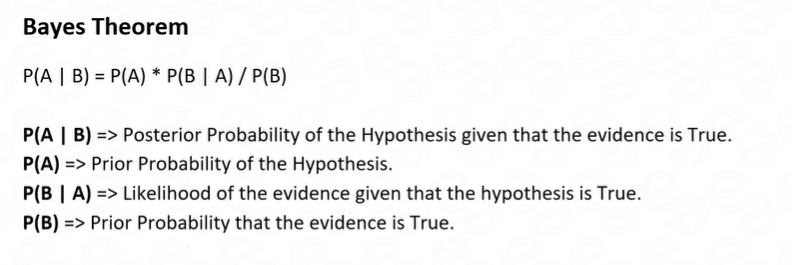
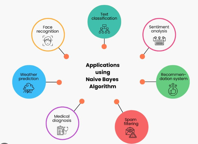
The Naive Bayes algorithm is a supervised machine learning algorithm based on Bayes' theorem with an assumption of independence between features. It is widely used for classification tasks, especially in natural language processing and text classification.
Here's how the Naive Bayes algorithm works:
Step 1: Data Preparation
Start with a labeled dataset consisting of feature vectors and corresponding class labels.
Each feature vector represents an object or instance, and the class label indicates its category.
Step 2: Feature Selection
Identify the relevant features that are most important for the classification task.
These features should capture the characteristics of the data that are informative for distinguishing different classes.
Step 3: Training
Calculate the prior probabilities and conditional probabilities from the training dataset.
Prior probabilities represent the probability of each class label occurring in the dataset.
Conditional probabilities represent the probability of each feature value occurring given a particular class label.
Step 4: Prediction
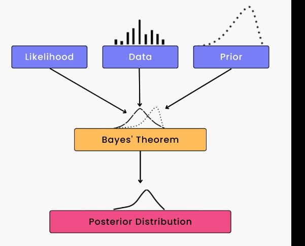
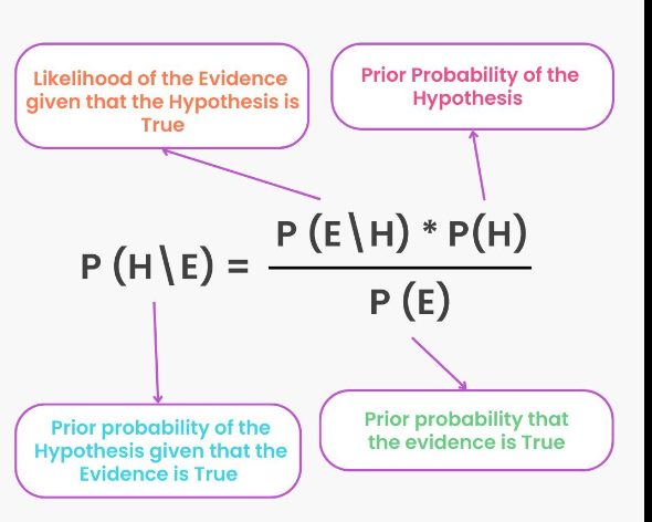
For a given test example, calculate the posterior probabilities for each class label using Bayes' theorem.
The posterior probability of a class label given the feature values is proportional to the product of the prior probability and the conditional probabilities.
The algorithm selects the class label with the highest posterior probability as the predicted class label for the test example.
Step 5: Evaluation
Assess the performance of the algorithm by comparing the predicted class labels with the true class labels from a separate test dataset.
Common evaluation metrics include accuracy, precision, recall, F1 score, or confusion matrix, depending on the task.
Example:
Let's consider a binary text classification problem to determine whether an email is spam or not based on the presence of certain keywords. We have a training dataset with the following feature vectors and labels:
Now, let's say we want to classify a new email with the feature values: "Free" = 1, "Discount" = 1, "Money" = 0. We can apply the Naive Bayes algorithm as follows:
Step 1: Data Preparation and Feature Selection: Already done with the provided dataset.
Step 2: Training:
Calculate the prior probabilities: P(Spam) = 0.5 and P(Not Spam) = 0.5 (assuming equal class distribution).
Calculate the conditional probabilities for each feature:
P("Free" = 1 | Spam) = 0.5
P("Discount" = 1 | Spam) = 0.5
P("Money" = 1 | Spam) = 0.5
P("Free" = 1 | Not Spam) = 0.5
P("Discount" = 1 | Not Spam) = 1.0
P("Money" = 1 | Not Spam) = 0.5
Step 4: Prediction:
Calculate the posterior probabilities for each class label:
P(Spam | "Free" = 1, "Discount" = 1, "Money" = 0) ∝ P("Free" = 1 | Spam) * P("Discount" = 1 | Spam) * P("Money" = 0 | Spam)
P(Spam | "Free" = 1, "Discount" = 1, "Money" = 0) ∝ 0.5 * 0.5 * (1 - 0.5) = 0.125
P(Not Spam | "Free" = 1, "Discount" = 1, "Money" = 0) ∝ P("Free" = 1 | Not Spam) * P("Discount" = 1 | Not Spam) * P("Money" = 0 | Not Spam)
= 0.5 * 1.0 * (1 - 0.5) = 0.25
Normalize the posterior probabilities to obtain the probabilities:
P(Spam | "Free" = 1, "Discount" = 1, "Money" = 0) = 0.125 / (0.125 + 0.25) = 0.333
P(Not Spam | "Free" = 1, "Discount" = 1, "Money" = 0) = 0.25 / (0.125 + 0.25) = 0.667
Based on the highest probability, the Naive Bayes algorithm predicts that the new email is "Not Spam."
Step 5: Evaluation:
Compare the predicted class label with the true class label from a test dataset to assess the performance of the algorithm.
Output:
In the provided example, the Naive Bayes algorithm predicts that the new email with the feature values "Free" = 1, "Discount" = 1, "Money" = 0 is classified as "Not Spam."
Please note that this is a simplified example for illustration purposes, and in practice, Naive Bayes algorithms can handle multiple features and larger datasets with more sophisticated probability estimations.




Top comments (0)