what is bais
Methods to solve bais and variance
Explain bais trade off
when data set imbalanced in machine learnings
When hyperparameter tunning is used
Explain hyperparameter Tunning Methods
Bias
refers to the error introduced by approximating a real-world problem with a simplified model. It represents the model's tendency to consistently underfit or oversimplify the underlying patterns in the data. A high bias model pays little attention to the training data and makes strong assumptions, which can lead to significant errors even on the training set.
For example, let's consider a regression problem where we want to predict housing prices based on the number of bedrooms. If we use a linear regression model to predict the prices but assume a simple relationship where the price is only dependent on the number of bedrooms, we may introduce bias. This simplified model may fail to capture other relevant features such as square footage or location, resulting in a high bias and poor performance.
Variance
on the other hand, refers to the model's sensitivity to fluctuations in the training data. It represents the model's tendency to overfit or be excessively complex, c*apturing noise and random fluctuations in the training set* that may not exist in the underlying true relationship. A high variance model adapts too much to the training data, resulting in poor generalization to new, unseen data.
Continuing with the housing price prediction example, let's suppose we use a highly flexible model such as a deep neural network with numerous layers and parameters. If we have limited training data and train the neural network for an extended period, it may memorize the training set, including its noise or outliers. Such a model will have low training error but high variance, performing poorly on new data.
To better understand the difference between bias and variance, let's consider their effects on the model's performance.
High Bias, Low Variance:
Training Set Error: High
Test Set Error: High
Example: A simple linear regression model that assumes a linear relationship between features and target variable, but the true relationship is more complex.
Low Bias, High Variance:
Training Set Error: Low
Test Set Error: High
Example: A decision tree with many branches that perfectly fits the training data, including noise or outliers.
To balance bias and variance and achieve better overall performance, it is important to consider regularization techniques. Regularization methods like L1 or L2 regularization and early stopping can help mitigate the model's complexity and address high variance. On the other hand, increasing model complexity, adding more features, or using more advanced algorithms can help reduce bias.
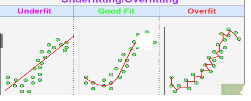
In machine learning, underfitting and overfitting are two common problems that can occur when building predictive models. They are opposite issues that arise when the model fails to generalize well from the training data to new, unseen data.
Underfitting
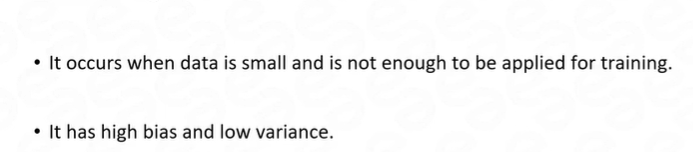
It occurs when a model is too simple or lacks the capacity to capture the underlying patterns in the data. It occurs when the model is not able to fit the training data well and, as a result, also performs poorly on unseen data. Underfitting can happen when the model is too constrained, has too few features, or is not trained for a sufficient number of iterations.
For example, let's consider a regression problem where we want to predict housing prices based on the number of bedrooms. If we use a linear model that can only fit a straight line to the data, it may underfit the data if the relationship between the number of bedrooms and the house prices is more complex than a simple linear relationship. In this case, the model would not capture the nuances of the data, resulting in poor performance both on the training set and new data.
Overfitting
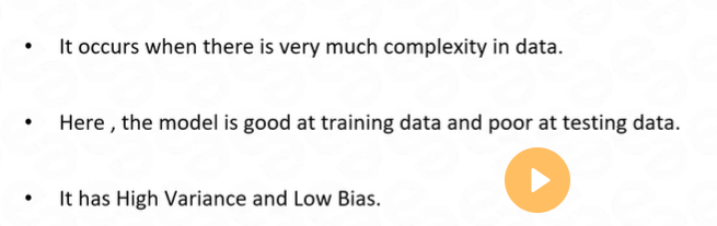
on the other hand, occurs when a model is too complex or overly flexible, and it learns the noise or random fluctuations in the training data instead of the underlying patterns. In other words, the model becomes too specific to the training data and fails to generalize well to new, unseen data. Overfitting can happen when the model has too many features, is too flexible, or is trained for too long.
Continuing with the housing price prediction example, let's suppose we have a large dataset with various features such as the number of bedrooms, square footage, location, and even noise level. If we use a highly complex model such as a decision tree with many branches, it may learn to fit the training data extremely well, including all the noise or outliers specific to the training set. However, when presented with new data, the overfitted model is likely to perform poorly because it learned the noise instead of the true underlying patterns.
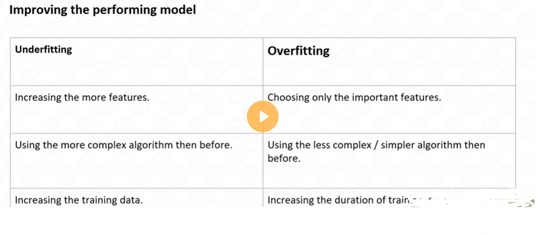
To address these issues, it is crucial to find the right balance between model simplicity and complexity. Underfitting can be mitigated by using more powerful models or adding more relevant features, while overfitting can be tackled by using regularization techniques, such as adding penalties to complex models or using techniques like cross-validation to evaluate model performance.
Hyperparameter
In machine learning, hyperparameters are parameters that are set before the learning process begins. They define the behavior and characteristics of a model and cannot be learned from the data itself. These parameters control various aspects of the learning algorithm, such as the model's complexity, regularization, and optimization process.
Here's an example to illustrate the concept of hyperparameters in machine learning:
Let's consider a popular algorithm called Support Vector Machines (SVM) for binary classification. Some of the hyperparameters for SVM include:
Kernel: SVM uses a kernel function to transform the input data into a higher-dimensional feature space. Common choices for the kernel are linear, polynomial, or radial basis function (RBF). The choice of kernel affects the model's ability to capture complex relationships in the data.
Regularization parameter (C): This parameter determines the trade-off between achieving a low training error and keeping the model's complexity low. Higher values of C allow the model to fit the training data more closely, potentially leading to overfitting.
Kernel coefficient (gamma): This parameter is specific to certain kernel functions, such as RBF. It defines the influence of each training example in the decision boundary. Higher values of gamma result in a more complex decision boundary.
Now, let's implement a simple SVM model with hyperparameter tuning in a Django application. We'll use the scikit-learn library for machine learning:
Install scikit-learn: Run pip install scikit-learn in your Django project's virtual environment.
Create a view function in your Django app's views.py file:
from django.shortcuts import render
from sklearn import svm
from sklearn.datasets import make_classification
from sklearn.model_selection import GridSearchCV

def svm_classification(request):
    # Generate some example data
    X, y = make_classification(n_samples=100, n_features=2, n_informative=2,
                               n_redundant=0, random_state=42)

    # Define the parameter grid for hyperparameter tuning
    param_grid = {'C': [0.1, 1, 10], 'gamma': [0.1, 1, 10], 'kernel': ['linear', 'rbf']}

    # Create an SVM classifier
    svm_model = svm.SVC()

    # Perform grid search for hyperparameter tuning
    grid_search = GridSearchCV(svm_model, param_grid, cv=3)
    grid_search.fit(X, y)

    # Get the best hyperparameters
    best_params = grid_search.best_params_

    # Fit the model with the best hyperparameters
    svm_model_best = svm.SVC(**best_params)
    svm_model_best.fit(X, y)

    # Make predictions
    test_data = [[-0.5, 0.5], [0.5, -0.5]]
    predictions = svm_model_best.predict(test_data)

    # Prepare the output
    context = {'best_params': best_params, 'predictions': predictions}
    return render(request, 'svm_classification.html', context)
Create a template file named svm_classification.html in your app's templates directory:
<html>
<head>
    <title>SVM Classification</title>
</head>
<body>
    <h1>Best Hyperparameters: {{ best_params }}</h1>
    <h2>Predictions: {{ predictions }}</h2>
</body>
</html>
How to solve Overfitting Problem
Overfitting is a common problem in machine learning where a model performs well on the training data but f*ails to generalize well on unseen data. It occurs when a **model learns the noise and irrelevant patterns* in the training data, resulting in poor performance on new data.
To address overfitting, you can consider the following approaches:
Increase Training Data: Adding more diverse and representative data to the training set can help the model learn better and generalize well. With more data, the model can capture the underlying patterns instead of overfitting to specific instances.
Feature Selection: Choose relevant and informative features for the model training. Remove any irrelevant or redundant features that may introduce noise or bias. Feature selection techniques like correlation analysis or domain knowledge can be used to identify important features.
Regularization: Regularization techniques add a penalty term to the model's objective function, discouraging overly complex models. Two common regularization techniques are L1 regularization (Lasso) and L2 regularization (Ridge). They help control the model's complexity and prevent overfitting.
Cross-Validation: Instead of evaluating the model's performance solely on the training set, use cross-validation techniques like k-fold cross-validation. It helps estimate the model's performance on unseen data by splitting the data into multiple subsets and performing training and validation iterations.
Early Stopping: Monitor the model's performance during training and stop training early if the performance on a validation set starts to degrade. This prevents the model from overfitting by avoiding unnecessary training epochs.
Ensemble Methods: Combine multiple models to make predictions. Ensemble methods like bagging (e.g., Random Forest) and boosting (e.g., Gradient Boosting) help reduce overfitting by combining the predictions of multiple weak models into a stronger and more generalized model.
Example:
Let's consider a scenario where you have a classification problem. You train a deep neural network on a small dataset and observe that the model overfits. To address overfitting, you can apply the following techniques:
Increase Training Data: Collect more labeled samples from different sources or use data augmentation techniques to generate additional training data by applying transformations like rotations, translations, or flips to existing samples.
Regularization: Apply L2 regularization to the model by adding a weight decay term to the loss function. This helps prevent excessive weights and encourages the model to focus on important features.
Dropout: Add dropout layers to the network architecture. Dropout randomly deactivates a certain percentage of neurons during training, forcing the network to rely on different combinations of features and reducing the likelihood of overfitting.
Early Stopping: Monitor the validation loss during training and stop training when the loss starts to increase or reaches a predefined threshold. This prevents the model from overfitting to the training data by finding the optimal balance between underfitting and overfitting.
By implementing these techniques, you can address overfitting and improve the model's generalization performance on unseen data. It's important to experiment with different approaches and evaluate their impact on the model's performance to find the most effective solution for your specific problem.
When hyperparameter tunning is used
Hyperparameter tuning is used in machine learning to find the best configuration of hyperparameters for a given model. Hyperparameters are parameters that are set before training the model and are not learned during the training process. They control the behavior and complexity of the model, and choosing the right values for hyperparameters can significantly impact the model's performance.
Hyperparameter tuning is necessary because different hyperparameter settings can lead to different model behavior and performance. The goal is to f*ind the optimal combination of hyperparameters* that results in the best performance on the validation or test dataset.
Hyperparameter tuning is typically performed after the initial model is constructed and before it is deployed for real-world use. It involves the following steps:
Define the Hyperparameter Search Space: Determine the range or possible values for each hyperparameter that you want to tune. This could be a discrete set of values or a continuous range.
Choose a Search Method: Select a method for exploring the hyperparameter search space. Common search methods include Grid Search, Random Search, Bayesian Optimization, Genetic Algorithms, and more.
Split Data into Training and Validation Sets: To evaluate different hyperparameter configurations, the dataset is divided into training and validation sets. The model is trained on the training set and evaluated on the validation set.
Perform Hyperparameter Search: Run the selected search method to explore different hyperparameter combinations. The performance of the model is evaluated for each combination on the validation set.
Select Best Hyperparameters: Once the hyperparameter search is complete, choose the hyperparameter configuration that results in the best performance on the validation set.
Evaluate Model Performance: After obtaining the best hyperparameters, the model is retrained on the entire training dataset (including the validation set) and evaluated on a separate test set to assess its performance on new, unseen data.
Hyperparameter tuning is crucial for improving model performance and generalization. It can help avoid overfitting and underfitting and lead to a model that performs well on a wide range of datasets. However, hyperparameter tuning can be computationally expensive and time-consuming, especially when using exhaustive search methods like Grid Search. Therefore, it's essential to balance the computational cost with the potential improvement in performance when deciding the scope of the hyperparameter search.
Methods to solve bais and variance
To solve the bias-variance trade-off and build a model that performs well on both training and new, unseen data, you can use various techniques to reduce bias and variance. Here are some methods to address bias and variance:
1. Adjusting Model Complexity:
High Bias (Underfitting): If your model has high bias and is underfitting the data, you can increase the model's complexity. This can involve using a more complex algorithm, adding more features, or increasing the degree of polynomial regression.
High Variance (Overfitting): If your model has high variance and is overfitting the data, you can reduce the model's complexity. This can be done using techniques like regularization (e.g., L1 or L2 regularization for linear models), feature selection, or using simpler algorithms.
2. Cross-Validation:
Cross-validation is a valuable technique to estimate how well your model will generalize to new data. It helps you tune hyperparameters and assess the model's performance on unseen data. By using techniques like k-fold cross-validation, you can get a better sense of your model's bias and variance and choose appropriate hyperparameters that strike the right balance.
3. Regularization:
Regularization methods can help you control the model's complexity and reduce variance. For example, in linear regression, L1 (Lasso) or L2 (Ridge) regularization can be used to penalize large coefficients and prevent overfitting.
4. Ensemble Methods:
Ensemble methods combine multiple models to reduce variance and improve performance. Techniques like Bagging (Bootstrap Aggregating) and Boosting (e.g., AdaBoost, Gradient Boosting) create an ensemble of weak learners, which can lead to a more robust and accurate model.
5. Feature Engineering and Selection:
Carefully selecting or engineering features can improve a model's performance and reduce overfitting. Removing irrelevant or noisy features can help the model focus on the most important information.
6. Data Augmentation:
For small datasets, data augmentation techniques can be used to artificially increase the training set size by creating slightly modified copies of the existing data. This can help the model learn more robust and generalizable patterns.
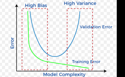
7. Bias-Variance Analysis:
Understanding the bias-variance trade-off through analysis of learning curves or bias-variance plots can provide insights into your model's behavior and guide you in making improvements.
It's important to note that addressing bias and variance is an iterative process. You may need to try different combinations of techniques and fine-tune hyperparameters to find the right balance for your specific problem and dataset. Regular monitoring and evaluation of the model's performance on both training and validation data are essential to ensure it is neither underfitting nor overfitting. By striking the right balance, you can build a model that generalizes well and provides accurate predictions for new, unseen data.
Explain bais trade off
The bias-variance trade-off is a fundamental concept in machine learning that deals with finding the right balance between bias and variance in a model to achieve optimal performance.
Bias represents the error introduced by a model's assumptions or simplifications about the underlying data. A high-bias model is often too simple and may not be able to capture the true complexity of the underlying data. This can result in underfitting, where the model performs poorly on both the training data and new, unseen data because it fails to learn the underlying patterns. Underfitting occurs when a model is not complex enough to represent the true relationship between input features and the target variable.
Variance represents the error introduced by a model's sensitivity to variations in the training data. A high-variance model is very flexible and can fit the training data very well, but it may fail to generalize to new, unseen data. This can lead to overfitting, where the model memorizes noise or random fluctuations in the training data, resulting in poor performance on new data. Overfitting occurs when a model is too complex and captures noise and idiosyncrasies in the training data rather than the general patterns.
The bias-variance trade-off arises because, as you try to reduce one type of error (bias or variance), the other tends to increase. Finding the optimal trade-off point is crucial to building a model that generalizes well to new data.
Low Bias, High Variance:
- Occurs when a model is very flexible and can fit the training data well.
- Tends to overfit and perform poorly on new data.
The model is sensitive to small variations in the training data
.
High Bias, Low Variance:Occurs when a model is too simple and cannot capture the underlying patterns in the data.
Tends to underfit and perform poorly on both training and new data.
The model does not adapt well to changes in the data
.
Balancing Bias and Variance:
To find the right balance, you can:Adjust Model Complexity: Increase model complexity to reduce bias (e.g., by adding more features or increasing the degree of polynomial regression) or decrease model complexity to reduce variance (e.g., by using regularization or feature selection).
Use Cross-Validation: Cross-validation helps to estimate how well a model will generalize to new data and allows you to fine-tune the model's complexity.
Ensemble Methods: Combine multiple models (e.g., using bagging or boosting) to reduce variance while maintaining or even reducing bias
.
The goal is to strike a balance that minimizes both bias and variance, leading to a model that performs well on both the training data and new, unseen data. This model will generalize well and provide more reliable predictions in real-world applications.
what is bais
In the context of machine learning and statistics, bias refers to the error or inaccuracy introduced by a model or estimator when attempting to approximate a target function or make predictions on new, unseen data. It is one of the key sources of error in a machine learning algorithm.
There are two main types of bias:
Bias (Underfitting): Bias occurs when a model is too simple to capture the underlying patterns and relationships in the data. A biased model tends to have low complexity and may overlook important features, resulting in a high training error. It often leads to poor performance on both the training data and the new, unseen data (test data) because the model cannot generalize well to different patterns.
Variance (Overfitting): Variance occurs when a model is too complex and highly sensitive to fluctuations in the training data. An overfit model learns the noise and random variations in the training data rather than the underlying patterns, leading to a very low training error but poor performance on new, unseen data. Overfitting can occur when a model tries to memorize the training data rather than learning the general patterns.
The goal in machine learning is to strike a balance between bias and variance to build a model that can generalize well to new data while capturing the relevant patterns from the training data. This trade-off is known as the bias-variance trade-off.
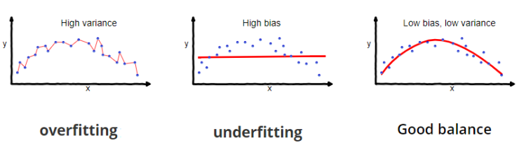
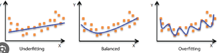
The bias-variance trade-off can be illustrated as follows:
A high-bias model tends to have low variance but high bias, leading to underfitting.
A high-variance model tends to have low bias but high variance, leading to overfitting.
To find the optimal model, you need to tune the hyperparameters and choose the appropriate model complexity that minimizes both bias and variance. Techniques like cross-validation and regularization can be used to mitigate overfitting and reduce bias. Regularization **methods, for example, penalize complex models** to avoid overfitting and find a balance between the two sources of error.
when data set imbalanced in machine learnings
An imbalanced dataset in machine learning refers to a situation where the distribution of class labels is not equal, leading to significantly more instances of one class compared to the other(s). Imbalanced datasets can be problematic for certain machine learning algorithms, as they tend to bias the model towards the majority class and may result in poor performance on the minority class. Here are some examples of imbalanced datasets:
Fraud Detection: In a credit card fraud detection problem, the majority of transactions are legitimate (non-fraudulent) with a very small proportion being fraudulent. The dataset will be heavily imbalanced, with the majority class being non-fraudulent transactions and the minority class being fraudulent transactions.
Medical Diagnosis: In medical diagnosis tasks, the occurrence of certain rare diseases might be significantly lower than common conditions. For instance, in a disease detection dataset, the majority class may represent healthy individuals, while the minority class represents patients with a rare disease.
Manufacturing Defect Detection: In a quality control scenario, most of the products might be defect-free (majority class), while only a small percentage have defects (minority class).
Customer Churn Prediction: When predicting customer churn in a subscription-based service, the majority of customers may continue their subscriptions, resulting in a smaller number of churn instances.
Anomaly Detection: In anomaly detection, the normal behavior of a system or process is the majority class, while the anomalies are the minority class.
Text Classification: In sentiment analysis, for instance, most of the user reviews might be positive, resulting in an imbalanced dataset with positive sentiment being the majority class.
Handling imbalanced datasets is essential to prevent the model from being biased and to achieve accurate predictions for both classes. S*ome techniques to address imbalanced datasets* include:
Resampling: This involves either oversampling the minority class by duplicating instances or undersampling **the majority class by **removing instances. Both methods aim to balance the class distribution.
Synthetic Data Generation: Techniques like Synthetic Minority Over-sampling Technique (SMOTE) create synthetic instances of the minority class to balance the dataset.
Class Weighting: Many machine learning algorithms allow you to assign different weights to classes, giving higher importance to the minority class during training.
Cost-Sensitive Learning: Modify the learning algorithm to consider the misclassification costs for different classes, encouraging it to prioritize the minority class.
Ensemble Methods: Ensemble techniques like Random Forest or AdaBoost can handle imbalanced datasets better than individual models.
Anomaly Detection Methods: For anomaly detection tasks, specialized algorithms like Isolation Forest or One-Class SVM can be more effective.
It's important to carefully choose the appropriate method for dealing with imbalanced datasets based on the specific problem and dataset characteristics to avoid overfitting or other unintended consequences. Additionally, evaluation metrics such as precision, recall, F1-score, and area under the receiver operating characteristic curve (AUC-ROC) are more informative for imbalanced datasets compared to accuracy.
Hyperparameter Tunning Methods
Hyperparameter tuning is a crucial step in machine learning model development where you search for the best combination of hyperparameters to optimize your model's performance. Hyperparameters are settings that are not learned during training but are determined before training begins. Grid Search and Randomized Search are two common techniques used for hyperparameter tuning.
Grid Search:
Grid Search involves exhaustively searching through a predefined set of hyperparameter values to find the best combination. It constructs a grid of a*ll possible hyperparameter combinations* and evaluates the model's performance using cross-validation for each combination. This method is straightforward but can be computationally expensive, especially when dealing with a large number of hyperparameters and their potential values.
Example:
Let's consider tuning two hyperparameters, the learning rate and the number of trees, for a gradient boosting algorithm:
Learning Rate: [0.1, 0.01, 0.001]
Number of Trees: [50, 100, 150]
Grid Search would involve evaluating the model using all possible combinations: (0.1, 50), (0.1, 100), (0.1, 150), (0.01, 50), (0.01, 100), (0.01, 150), (0.001, 50), (0.001, 100), and (0.001, 150). It then selects the combination that yields the best performance.
Randomized Search:
Randomized Search is similar to Grid Search, but instead of evaluating all possible combinations, it samples a fixed number of random combinations from the predefined hyperparameter space. This approach is beneficial when the hyperparameter space is vast, as it provides a balance between exploration and exploitation of hyperparameters. It's often faster than Grid Search, as it doesn't evaluate all combinations.
Example:
Continuing with the gradient boosting algorithm, let's say you have the same hyperparameter space:
Learning Rate: [0.1, 0.01, 0.001]
Number of Trees: [50, 100, 150]
In Randomized Search, you would randomly select a certain number of combinations to evaluate, such as (0.1, 100), (0.01, 50), (0.001, 150), etc. The advantage is that you're exploring a variety of combinations without evaluating every possible one.
In both methods, you typically perform cross-validation during the evaluation to ensure that the performance estimates are reliable and not just overfitting to the training data. These techniques help you find hyperparameters that generalize well to unseen data and improve your model's performance.
Remember that the choice between Grid Search and Randomized Search depends on the size of the hyperparameter space, available computing resources, and the time you can dedicate to tuning.
here's an example implementation of Grid Search with Cross-Validation (GridSearchCV) for hyperparameter tuning using Python and scikit-learn library:
from sklearn.model_selection import GridSearchCV
from sklearn.ensemble import RandomForestClassifier
from sklearn.datasets import load_iris

# Load dataset
iris = load_iris()
X = iris.data
y = iris.target

# Define hyperparameter grid
param_grid = {
    'n_estimators': [50, 100, 150],
    'max_depth': [None, 10, 20],
    'min_samples_split': [2, 5, 10]
}

# Initialize model
model = RandomForestClassifier()

# Initialize GridSearchCV
grid_search = GridSearchCV(model, param_grid, cv=5, scoring='accuracy')

# Fit the GridSearchCV
grid_search.fit(X, y)

# Print best parameters and corresponding accuracy score
print("Best Parameters:", grid_search.best_params_)
print("Best Accuracy:", grid_search.best_score_)
In this example, we're using the Iris dataset and a RandomForestClassifier as the base model. We define a grid of hyperparameters to search through (param_grid), including the number of trees, maximum depth, and minimum samples required to split a node. The GridSearchCV object performs cross-validation with 5 folds (cv=5) and uses accuracy as the scoring metric.
After fitting the GridSearchCV, you can access the best parameters and the corresponding accuracy score using grid_search.best_params_ and grid_search.best_score_.
Implementation of Randomized Search with Cross-Validation (RandomizedSearchCV) for hyperparameter tuning using Python and scikit-learn library:
from sklearn.model_selection import RandomizedSearchCV
from sklearn.ensemble import RandomForestClassifier
from sklearn.datasets import load_iris

# Load dataset
iris = load_iris()
X = iris.data
y = iris.target

# Define hyperparameter distributions
param_dist = {
    'n_estimators': [50, 100, 150, 200],
    'max_depth': [None, 10, 20, 30],
    'min_samples_split': [2, 5, 10],
    'min_samples_leaf': [1, 2, 4]
}

# Initialize model
model = RandomForestClassifier()

# Initialize RandomizedSearchCV
random_search = RandomizedSearchCV(model, param_distributions=param_dist, n_iter=10, cv=5, scoring='accuracy', random_state=42)

# Fit the RandomizedSearchCV
random_search.fit(X, y)

# Print best parameters and corresponding accuracy score
print("Best Parameters:", random_search.best_params_)
print("Best Accuracy:", random_search.best_score_)
In this example, we're again using the Iris dataset and a RandomForestClassifier as the base model. However, this time we define a distribution of hyperparameters (param_dist) instead of a fixed grid. The RandomizedSearchCV object performs random sampling from this distribution for a specified number of iterations (n_iter=10) and evaluates each combination using cross-validation with 5 folds (cv=5).
The other parts of the code are quite similar to the Grid Search example. After fitting the RandomizedSearchCV, you can access the best parameters and the corresponding accuracy score using random_search.best_params
Points and Objective Question
High bais ,low variance leads
low bais ,high variance leads
meaning of variance and bais
when bais and variance occur
when underfitting and overfitting occurs
solution of underfitting and overfitting by which technique
difference between underfitting and overfitting
how to overcome imbalnce dataset by technique
when imabalnced dataset occur
realtime example of imbalanced dataset
when hyparameter tunniing used
what are the hypermater tunning method
when randomized search method is used
what is grid search methods

Top comments (0)