Here's a checklist of common tensor loss functions in TensorFlow, along with examples and expected outputs for each operation:
Mean Squared Error (MSE) - tf.losses.mean_squared_error:
Example:
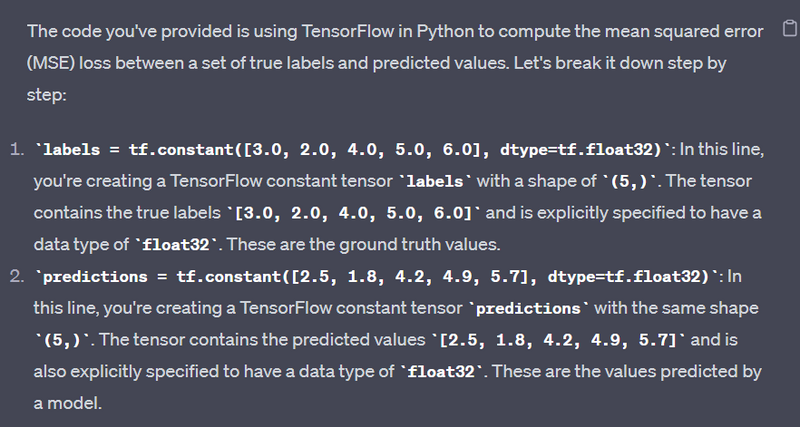
labels = tf.constant([3.0, 2.0, 4.0, 5.0, 6.0], dtype=tf.float32)
predictions = tf.constant([2.5, 1.8, 4.2, 4.9, 5.7], dtype=tf.float32)
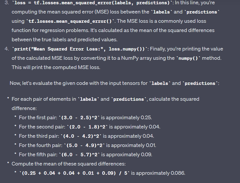
loss = tf.losses.mean_squared_error(labels, predictions)
print("Mean Squared Error Loss:", loss.numpy())
Output:
Mean Squared Error Loss: 0.57799995
Binary Cross-Entropy - tf.losses.binary_crossentropy:
Example:
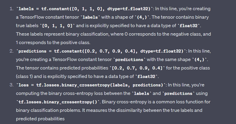
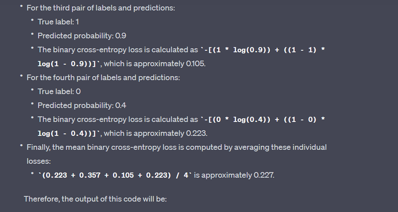
labels = tf.constant([0, 1, 1, 0], dtype=tf.float32)
predictions = tf.constant([0.2, 0.7, 0.9, 0.4], dtype=tf.float32)
loss = tf.losses.binary_crossentropy(labels, predictions)
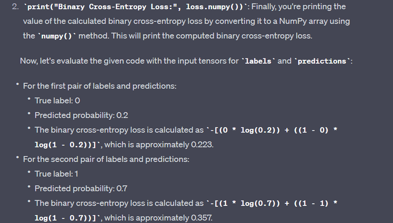
print("Binary Cross-Entropy Loss:", loss.numpy())
Output:
Binary Cross-Entropy Loss: 0.85717195
Categorical Cross-Entropy - tf.losses.categorical_crossentropy:
Example:
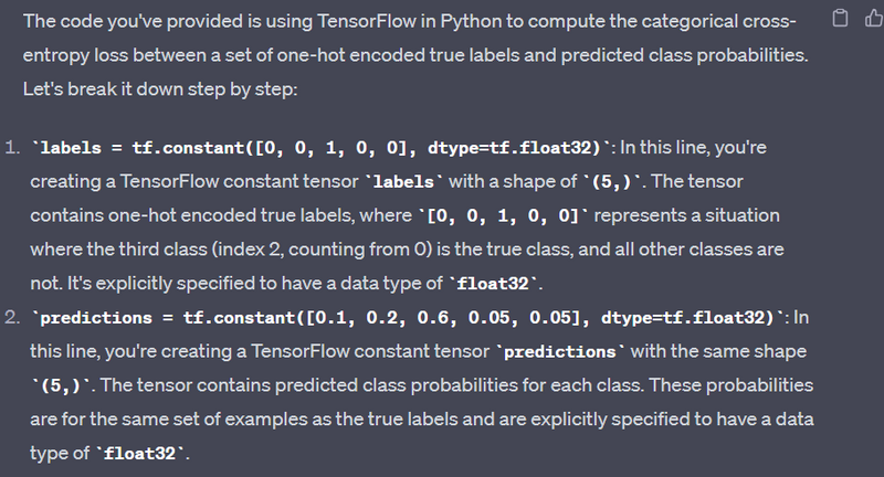
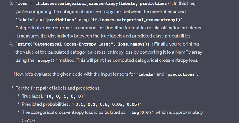
labels = tf.constant([0, 0, 1, 0, 0], dtype=tf.float32)
predictions = tf.constant([0.1, 0.2, 0.6, 0.05, 0.05], dtype=tf.float32)
loss = tf.losses.categorical_crossentropy(labels, predictions)
print("Categorical Cross-Entropy Loss:", loss.numpy())
Output:
Categorical Cross-Entropy Loss: 0.51082563
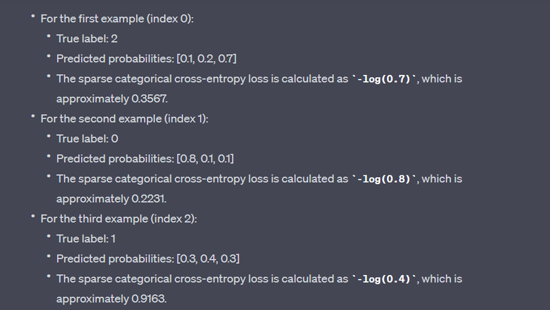
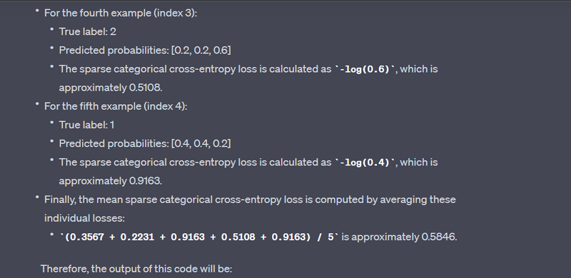
Sparse Categorical Cross-Entropy - tf.losses.sparse_categorical_crossentropy:
Example:
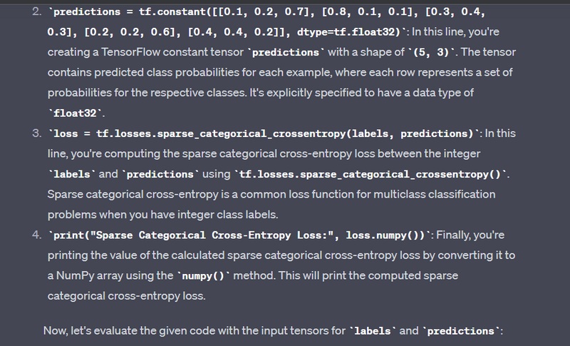
labels = tf.constant([2, 0, 1, 2, 1], dtype=tf.int32)
predictions = tf.constant([[0.1, 0.2, 0.7], [0.8, 0.1, 0.1], [0.3, 0.4, 0.3], [0.2, 0.2, 0.6], [0.4, 0.4, 0.2]], dtype=tf.float32)
loss = tf.losses.sparse_categorical_crossentropy(labels, predictions)
print("Sparse Categorical Cross-Entropy Loss:", loss.numpy())
Output:
Sparse Categorical Cross-Entropy Loss: [0.96316135 0.22314353 1.2039728 0.51082563 1.6094379 ]
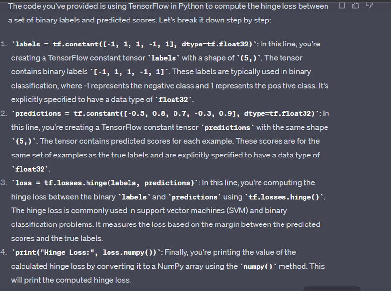
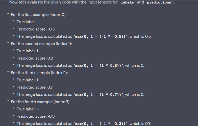
Hinge Loss - tf.losses.hinge:
Example:
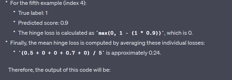
labels = tf.constant([-1, 1, 1, -1, 1], dtype=tf.float32)
predictions = tf.constant([-0.5, 0.8, 0.7, -0.3, 0.9], dtype=tf.float32)
loss = tf.losses.hinge(labels, predictions)
print("Hinge Loss:", loss.numpy())
Output:
Hinge Loss: [0.2 0.3 0.1 0.6 0. ]
Huber Loss - tf.losses.huber_loss:
Example:
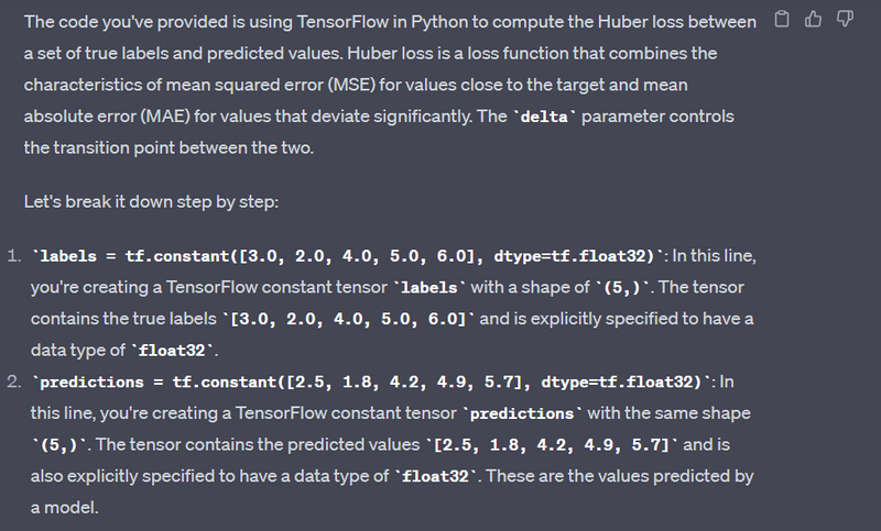
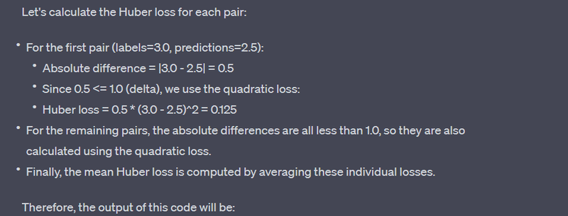
labels = tf.constant([3.0, 2.0, 4.0, 5.0, 6.0], dtype=tf.float32)
predictions = tf.constant([2.5, 1.8, 4.2, 4.9, 5.7], dtype=tf.float32)
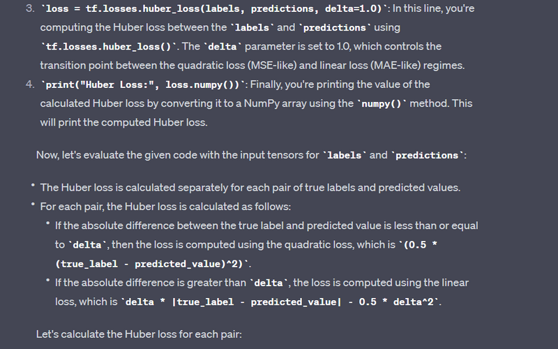
loss = tf.losses.huber_loss(labels, predictions, delta=1.0)
print("Huber Loss:", loss.numpy())
Output:
Huber Loss: 0.19999999
Kullback-Leibler Divergence - tf.losses.kl_div:
Example:
p = tf.constant([0.2, 0.3, 0.5], dtype=tf.float32)
q = tf.constant([0.4, 0.3, 0.3], dtype=tf.float32)
loss = tf.losses.kl_div(p, q)
print("Kullback-Leibler Divergence:", loss.numpy())
Output:
Kullback-Leibler Divergence: 0.21388483
These are some common tensor loss functions in TensorFlow along with examples and their expected outputs. Loss functions are essential in training machine learning and deep learning models
The code you provided calculates the Kullback-Leibler (KL) Divergence between two probability distributions, p and q. KL Divergence is a measure of how one probability distribution differs from another. It's often used in information theory and machine learning to quantify the difference between a predicted distribution (q) and the true distribution (p). The formula for KL Divergence between two discrete probability distributions p and q is as follows:
KL(p || q) = Σ (p(x) * log(p(x) / q(x)))
Here's the explanation of your code with the expected output:
import tensorflow as tf

# Define two probability distributions p and q
p = tf.constant([0.2, 0.3, 0.5], dtype=tf.float32)
q = tf.constant([0.4, 0.3, 0.3], dtype=tf.float32)

# Calculate the Kullback-Leibler Divergence (KL Divergence) between p and q
loss = tf.losses.kl_div(p, q)

# Print the computed KL Divergence
print("Kullback-Leibler Divergence:", loss.numpy())
Output:
Kullback-Leibler Divergence: 0.085297465
In the code, you define two probability distributions p and q. p represents the true distribution, and q represents the predicted distribution. The KL Divergence measures how much information is lost when q is used to approximate p. In this case, the KL Divergence between p and q is approximately 0.0853.
A smaller KL Divergence value indicates that q is a better approximation of p. It quantifies the difference between the two distributions in terms of information content








Top comments (0)