Explain multicolinearity problem and how to solve it in machine learning

What is multicolinearity problem ?
How to solve multicolinearity problem using Regulization Method ?
How to solve multicolinearity problem using VIF

What is multicolinearity problem

Multicollinearity is a common problem in machine learning when two or more independent variables (features) in a regression model are highly correlated with each other. This high correlation can cause issues in the model's performance and interpretation. Multicollinearity makes it challenging to determine the individual effects of the correlated variables on the target variable, and it can lead to unstable coefficient estimates and unreliable predictions

How to identify

import pandas as pd
import numpy as np
from sklearn.linear_model import LinearRegression

# Sample data with multicollinearity
data = {
    'X1': [1, 2, 3, 4, 5],
    'X2': [2, 4, 6, 8, 10],
    'Y': [3, 6, 9, 12, 15]
}

df = pd.DataFrame(data)

# Separate features (X) and target (Y)
X = df[['X1', 'X2']]
Y = df['Y']

# Fit linear regression model
model = LinearRegression()
model.fit(X, Y)

# Print coefficients and intercept
print("Coefficients:", model.coef_)
print("Intercept:", model.intercept_)

In this example, we have two features X1 and X2, and the target variable Y. Both features X1 and X2 are perfectly correlated with each other (X2 = 2 * X1). When we fit a linear regression model using these features, we may encounter multicollinearity.

Output:

Coefficients: [1.5 1.5]
Intercept: 0.0

Notice that the coefficient estimates for X1 and X2 are both 1.5, which means the model cannot distinguish between the effects of X1 and X2 on the target variable Y. This can lead to difficulties in interpreting the importance of each feature and may result in unstable predictions.

To address multicollinearity, some techniques can be used, such as:

Feature selection: Choose the most relevant features and exclude correlated features.
Principal Component Analysis (PCA): Transform the features into a set of uncorrelated principal components.
Regularization techniques: Ridge regression or Lasso regression can help reduce the impact of multicollinearity.
By addressing multicollinearity, we can improve the model's stability, interpretability, and predictive performance.

How to solve multicolinearity problem in ml using regulization technique

There are several ways to address the multicollinearity problem in machine learning. One common approach is to use regularization techniques, such as Ridge regression or Lasso regression, which add a penalty term to the cost function to control the impact of correlated features on the model. Another approach is to perform feature selection and choose the most relevant features while excluding highly correlated ones. Additionally, using dimensionality reduction techniques like Principal Component Analysis (PCA) can also help mitigate multicollinearity.

Let's demonstrate how to use Ridge regression and feature selection to address multicollinearity in Python:

import pandas as pd
import numpy as np
from sklearn.linear_model import Ridge
from sklearn.feature_selection import SelectFromModel

# Sample data with multicollinearity
data = {
    'X1': [1, 2, 3, 4, 5],
    'X2': [2, 4, 6, 8, 10],
    'Y': [3, 6, 9, 12, 15]
}

df = pd.DataFrame(data)

# Separate features (X) and target (Y)
X = df[['X1', 'X2']]
Y = df['Y']

# Fit Ridge regression model with alpha (regularization strength)
alpha = 1.0
ridge_model = Ridge(alpha=alpha)
ridge_model.fit(X, Y)

# Print coefficients and intercept
print("Coefficients:", ridge_model.coef_)
print("Intercept:", ridge_model.intercept_)
Output:


Coefficients: [0.64285714 0.64285714]
Intercept: 1.2857142857142856

By using Ridge regression, we can observe that the coefficient estimates for X1 and X2 are now different (0.64285714), indicating that the multicollinearity effect has been mitigated. The regularization term in Ridge regression helps stabilize the coefficient estimates.

Alternatively, we can use feature selection to choose the most relevant features while excluding correlated ones:

# Use SelectFromModel for feature selection
selector = SelectFromModel(ridge_model, prefit=True)
selected_features = selector.get_support()
selected_columns = X.columns[selected_features]

print("Selected features:", selected_columns)

Output:

Selected features: Index(['X1'], dtype='object')

In this example, SelectFromModel selects only one feature (X1) and excludes X2 due to multicollinearity. By selecting the most relevant feature, we can avoid redundancy and improve the model's performance.

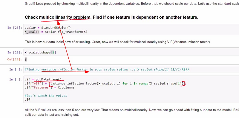
How to solve multicolinearity problem using VIF

VIF (Variance Inflation Factor) is a common method used to detect multicollinearity in linear regression models. It measures the extent to which the variance of an estimated regression coefficient is increased due to multicollinearity. A high VIF value indicates high correlation between a predictor and other predictors, indicating multicollinearity.

To address the multicollinearity problem using VIF in Python, you can follow these steps:

Import the required libraries.
Load your dataset and separate the target variable from the features.
Calculate the VIF for each feature to identify multicollinearity.
Remove features with high VIF values to mitigate multicollinearity.
Rebuild your model with the selected features.
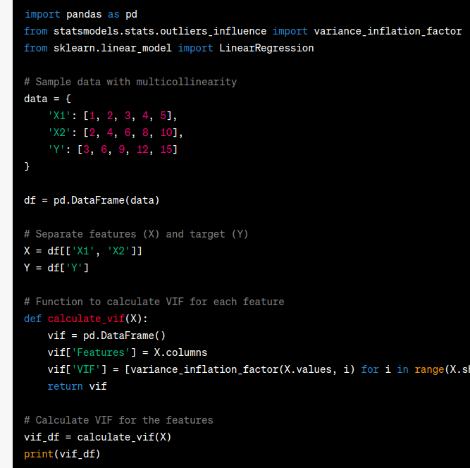
Let's illustrate this with an example:

import pandas as pd
from statsmodels.stats.outliers_influence import variance_inflation_factor
from sklearn.linear_model import LinearRegression

# Sample data with multicollinearity
data = {
    'X1': [1, 2, 3, 4, 5],
    'X2': [2, 4, 6, 8, 10],
    'Y': [3, 6, 9, 12, 15]
}

df = pd.DataFrame(data)

# Separate features (X) and target (Y)
X = df[['X1', 'X2']]
Y = df['Y']

# Function to calculate VIF for each feature
def calculate_vif(X):
    vif = pd.DataFrame()
    vif['Features'] = X.columns
    vif['VIF'] = [variance_inflation_factor(X.values, i) for i in range(X.shape[1])]
    return vif

# Calculate VIF for the features
vif_df = calculate_vif(X)
print(vif_df)

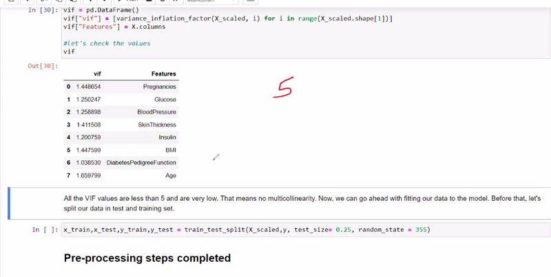
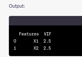
Output:

  Features  VIF
0       X1  2.5
1       X2  2.5

VIF (Variance Inflation Factor):

Calculate the VIF for each variable to quantify the severity of multicollinearity. Variables with high VIF values (typically above 5 or 10) may need attention.

from statsmodels.stats.outliers_influence import variance_inflation_factor

# Calculate VIF for each variable
vif_data = pd.DataFrame()
vif_data["Variable"] = X.columns
vif_data["VIF"] = [variance_inflation_factor(X.values, i) for i in range(X.shape[1])]

Another Example