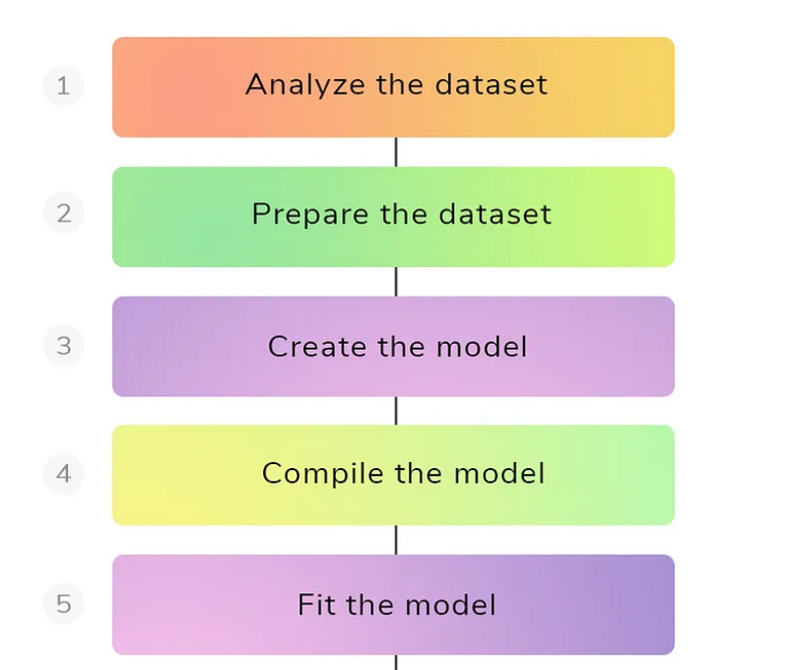
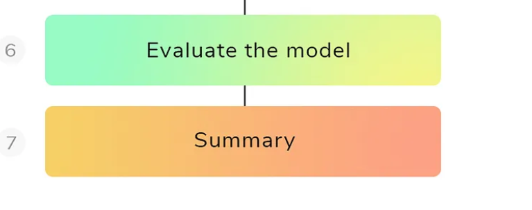
Basics models go through the following pipeline

Training Operations in tensor flow

Basics models go through the following pipeline

TensorFlow is a numerical processing library was originally developed at Google used by researchers and machine learning practitioners to conduct machine learning research. You can perform any numerical operation with TensorFlow, it is mostly used to train and run deep neural networks.

A simple computer vision model using Keras
Let’s start with a classical example of computer vision — digit recognition with the Modified National Institute of Standards and Technology (MNIST) datasets.

For installation of TensorFlow 2.x version.

#!pip install tensorflow==2.0.0alpha0 #Tensorflow alpha version
#!pip install tensorflow==2.0.0-beta1 #Tensorflow beta version
#print(tf.__version__) # Check the version

Preparing the data
First, we import the data. It is made up of 60,000 images for the training set and 10,000 images for the test set:

import tensorflow as tf # import tensorflow as tf for faster typing

import numpy as np      # import numerical python as np 
num_classes = 10
img_rows, img_cols = 28, 28
num_channels = 1
input_shape = (img_rows, img_cols, num_channels)
(x_train, y_train),(x_test, y_test) =  tf.keras.datasets.mnist.load_data()     #load the datasets
x_train, x_test = x_train / 255.0, x_test / 255.0 

DataNormalization

The tf.keras.datasets module provides quick access to download and instantiate a number of classical datasets. After importing the data using load_data, we divide the array by 255.0 to get a number in the range [0, 1] instead of [0, 255]. It is common practice to normalize data, either in the [0, 1] range or in the [-1, 1] range.

Building the model
Moving to building the actual model. We will use a very simple architecture composed of two fully connected layers called as Dense layers . Now, let’s have a look at the code. As you can see, Keras code is very briefly and clearly written.

model = tf.keras.models.Sequential()
model.add(tf.keras.layers.Flatten())
model.add(tf.keras.layers.Dense(128, activation='relu'))
model.add(tf.keras.layers.Dense(num_classes, activation='softmax'))

Since our model is a linear stack of layers, we start by calling the Sequential function. We then add each layer one after the other. Our model is composed of two fully connected layers. We build it layer by layer:

Flatten: This will take the 2D matrix representing the image pixels and turn it into a 1D array. We need to do this before adding a fully connected layer. The 28 × 28 images are turned into a vector of size 784.
Dense of size 128: This will turn the 784 pixel values into 128 activations using a weight matrix of size 128 × 784 and a bias matrix of size 128. In total, this means 100,480 parameters.
Dense of size 10: This will turn the 128 activations into our final prediction. Notice that because we want probabilities to sum to 1, we will use the softmax activation function. The softmax function takes the output of a layer and returns probabilities that sum up to 1. It is the activation of choice for the last layer of a classification model.
You can get a description of the model, the outputs, and their weights.

model.summary()

Here is the output:

Model: "sequential"
_________________________________________________________________
Layer (type) Output Shape Param # 
=================================================================
flatten_1 (Flatten) (None, 784) 0 
_________________________________________________________________
dense_1 (Dense) (None, 128) 100480 
_________________________________________________________________
dense_2 (Dense) (None, 10) 1290 
=================================================================
Total params: 101,770
Trainable params: 101,770
Non-trainable params: 0

Training the model
Keras makes training extremely simple:

model.compile(optimizer='sgd',loss='sparse_categorical_crossentropy, metrics=['accuracy'])

Calling .compile() on the model we just created is a mandatory step. A few arguments must be specified:

optimizer: This is the component that will perform the gradient descent.
loss: This is the metric we will optimize. In our case, we choose cross-entropy, just like in the previous chapter.
metrics: These are additional metric functions evaluated during training to provide further visibility of the model’s performance (unlike loss, they are not used in the optimization process).

model.fit(x_train, y_train, epochs=5, verbose=1, validation_data=(x_test, y_test))

Then, we call the .fit() method. We will train for five epochs, meaning that we will iterate over the whole train dataset five times. Notice that we set verbose to 1. This will allow us to get a progress bar with the metrics we chose earlier, the loss, and the Estimated Time of Arrival (ETA). The ETA is an estimate of the remaining time before the end of the epoch. Here is what the progress bar looks like:

Evaluate the model:

model.evaluate(x_test,y_test)

We followed three main steps:

Loading the data: In this case, the dataset was already available. During future projects, you may need additional steps to gather and clean the data.
Creating the model: This step was made easy by using Keras — we defined the architecture of the model by adding sequential layers. Then, we selected a loss, an optimizer, and a metric to monitor.
Training the model: Our model worked pretty well the first time. On more complex datasets, you will usually need to fine-tune parameters during training.

Training Operations in tensor flow

In TensorFlow, tensor training operations are operations specifically designed for training machine learning models. These operations involve the computation of gradients, optimization, and updating of model parameters based on the computed gradients. Training operations are a fundamental part of the training loop in machine learning, where the goal is to iteratively adjust model parameters to minimize a defined loss function.

Here are some key components and operations related to training in TensorFlow:

Loss Function:

The loss function measures the difference between the model's predictions and the actual target values. During training, the goal is to minimize this loss.
Example:

loss = tf.keras.losses.MeanSquaredError()(y_true, y_pred)

Gradients:

Gradients represent the rate of change of the loss with respect to the model parameters. TensorFlow's tf.GradientTape is commonly used to compute gradients during the training process.
Example:

with tf.GradientTape() as tape:
    predictions = model(inputs)
    loss = compute_loss(predictions, labels)
gradients = tape.gradient(loss, model.trainable_variables)

Optimizers:

Optimizers are algorithms that use gradients to update the model's parameters in the direction that reduces the loss. Common optimizers include SGD (Stochastic Gradient Descent), Adam, and RMSprop.
Example:

optimizer = tf.keras.optimizers.Adam(learning_rate=0.001)
optimizer.apply_gradients(zip(gradients, model.trainable_variables))

Training Step:

The training step typically involves forward pass, backward pass (computing gradients), and optimizer step (updating model parameters).
Example:

with tf.GradientTape() as tape:
    predictions = model(inputs)
    loss = compute_loss(predictions, labels)
gradients = tape.gradient(loss, model.trainable_variables)
optimizer.apply_gradients(zip(gradients, model.trainable_variables))

Epochs and Batches:

Training is usually done in epochs, where the entire dataset is passed through the model. Each epoch consists of multiple batches, and the model parameters are updated after processing each batch.
Example (using tf.data.Dataset):

dataset = tf.data.Dataset.from_tensor_slices((inputs, labels)).batch(batch_size)
for epoch in range(num_epochs):
    for batch_inputs, batch_labels in dataset:
        # Training step for each batch

Metrics:

Metrics are additional measurements used to evaluate the model's performance during training. Common metrics include accuracy, precision, and recall.
Example:

accuracy_metric = tf.keras.metrics.Accuracy()
accuracy_metric.update_state(labels, predictions)

Callbacks:

Callbacks are functions that can be applied at various points during training. They can be used for saving checkpoints, early stopping, or logging training progress.
Example:

callbacks = [
    tf.keras.callbacks.ModelCheckpoint(filepath='model_checkpoint.h5', save_best_only=True),
    tf.keras.callbacks.EarlyStopping(patience=3)
]
model.fit(inputs, labels, epochs=num_epochs, callbacks=callbacks)

In summary, tensor training operations in TensorFlow involve a combination of loss computation, gradient computation, optimization, and iterating through the dataset in epochs and batches.

reference