How the PyTorch nn Module Builds Neural Networks Automatically"

What is torch.nn?
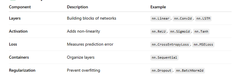
Key Components of nn module
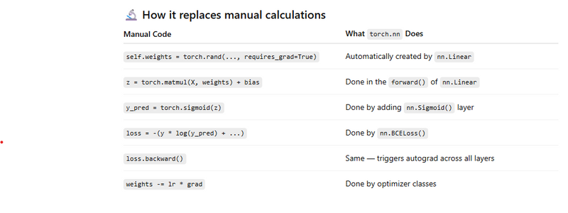
Comparsion of manual task and nn module with coding
Create neural network with hidden layer using nn module
Advantage of nn.sequential netwok to create layers
How to use builtin loss and built in optimizer
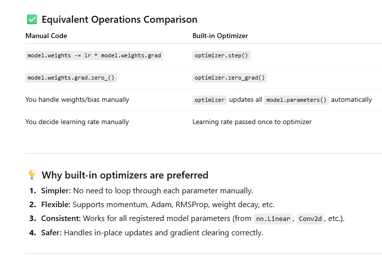
Difference between manual gradient descent and PyTorch’s built-in optimizers

What is torch.nn?
It is the core building block for creating and training neural networks easily without manually defining weights, biases, and formulas.

Let’s break it down with simple explanations, math, and how it replaces manual calculations.

What is torch.nn?

torch.nn is the Neural Network module of PyTorch.
It provides:

Pre-built layers (like nn.Linear, nn.Conv2d)

Activation functions (like nn.ReLU, nn.Sigmoid)

Loss functions (like nn.CrossEntropyLoss, nn.MSELoss)

Containers (nn.Sequential)

Regularization tools (nn.Dropout, nn.BatchNorm2d)

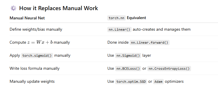
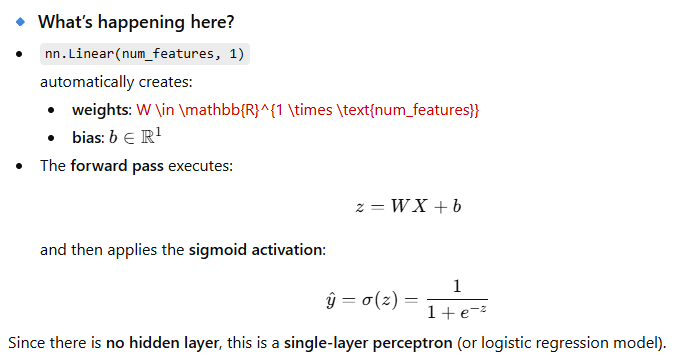
It abstracts away manual coding of weights, bias, and math like

Key Components of nn module

The torch.nn module in PyTorch is a core library that provides a wide array of classes and functions designed to help developers build neural networks efficiently and effectively.

It abstracts the complexity of creating and training neural networks by offering pre-built layers, loss functions, activation functions, and other utilities, enabling developers to focus on model design and experimentation rather than manual mathematical computations.

🔹

Key Components of torch.nn

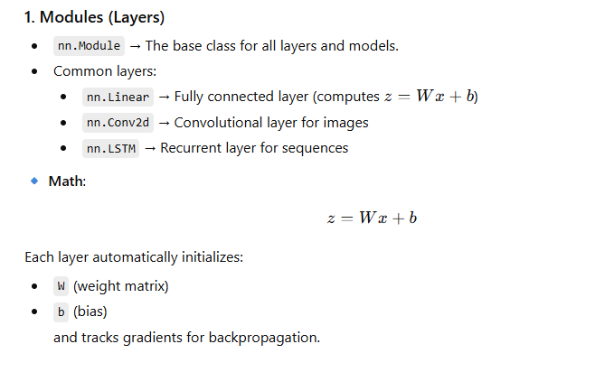
1. Modules (Layers):

nn.Module:
The base class for all neural network modules.
Every custom model or layer should subclass this class.

Common Layers include:

nn.Linear → Fully connected (dense) layer

nn.Conv2d → Convolutional layer (used for images)

nn.LSTM → Recurrent layer (used for sequential data like text or time series)

Each layer automatically manages its weights and biases, and PyTorch handles gradient calculations during training.

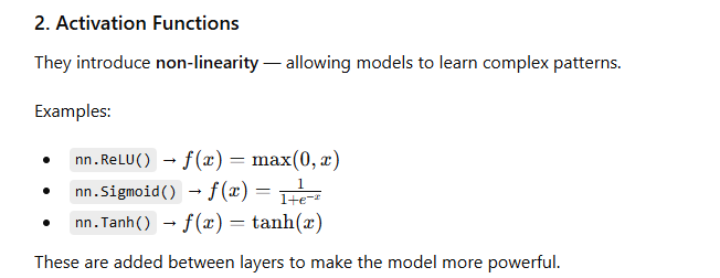
1. Activation Functions:

Functions that introduce non-linearity into the model, helping it learn complex relationships between input and output data.

Common examples:

nn.ReLU() → Rectified Linear Unit, outputs max(0, x)

nn.Sigmoid() → Converts values to range (0, 1)

nn.Tanh() → Converts values to range (-1, 1)

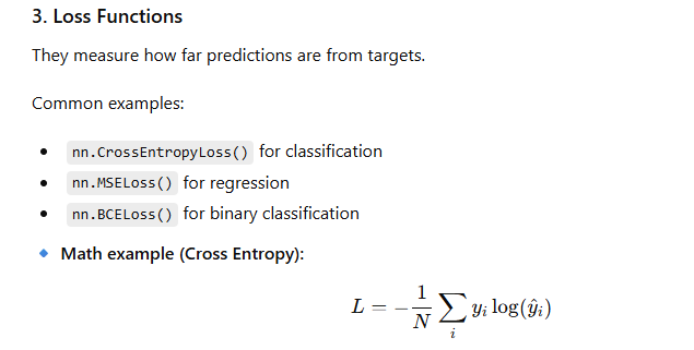
1. Loss Functions:

Loss functions measure how far the model’s predictions are from the actual values.

Common examples:

nn.CrossEntropyLoss() → Used for classification problems

nn.MSELoss() → Mean Squared Error, used for regression

nn.NLLLoss() → Negative Log Likelihood Loss, used with log-probabilities

These functions help quantify model errors so that optimization algorithms can minimize them.

1. Container Modules:

nn.Sequential:
A simple container that allows you to stack layers sequentially in order.
Example:

model = nn.Sequential(
    nn.Linear(3, 4),
    nn.ReLU(),
    nn.Linear(4, 1)
)

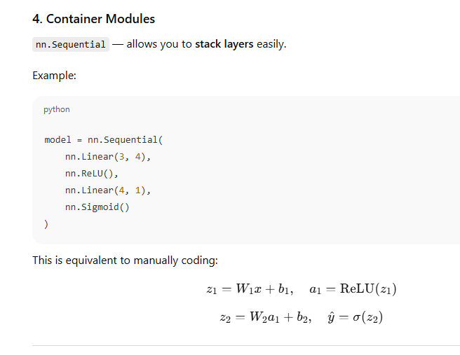
This simplifies building feedforward neural networks.

1. Regularization and Dropout:

These techniques help prevent overfitting and improve a model’s ability to generalize to new data.

Common examples:

nn.Dropout(p) → Randomly disables neurons during training with probability p

nn.BatchNorm2d() → Normalizes intermediate outputs, speeding up training and improving stability

Using your manual math (hand-written version)
import torch

X = torch.randn(4, 3)
W = torch.randn(3, 2, requires_grad=True)
b = torch.randn(2, requires_grad=True)

z = X @ W + b     # Linear transformation
y_pred = torch.sigmoid(z)  # Activation
loss = -(torch.log(y_pred)).mean()
loss.backward()   # Computes gradients manually

✅ Using torch.nn

import torch
import torch.nn as nn

# 1) Define model using nn.Module
model = nn.Sequential(
    nn.Linear(3, 2),     # Automatically creates W (3x2) and b (2,)
    nn.Sigmoid()         # Adds activation
)

# 2) Define loss
criterion = nn.BCELoss()

# 3) Example inputs and labels
X = torch.randn(4, 3)
y = torch.rand(4, 2)

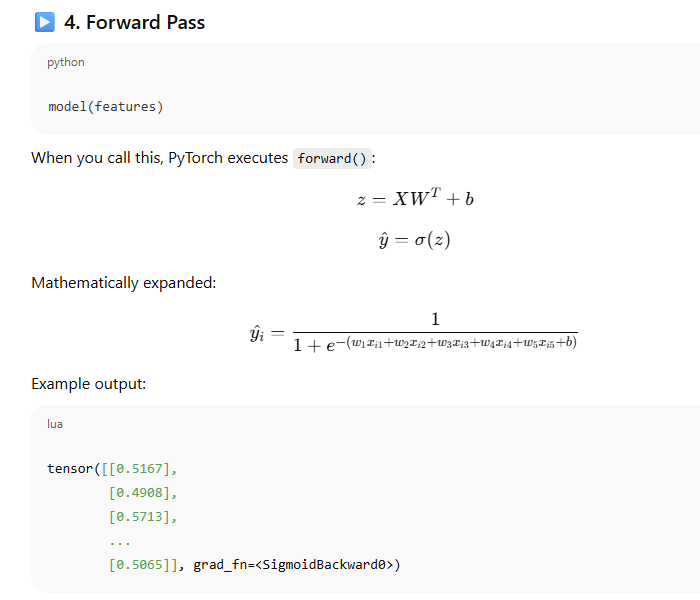
# 4) Forward pass
y_pred = model(X)

# 5) Compute loss
loss = criterion(y_pred, y)

# 6) Backpropagation
loss.backward()

Comparsion of manual task and nn module with coding

Manual Implementation (Before nn.Module)

import torch

# Manual weight and bias
W = torch.randn(num_features, 1, requires_grad=True)
b = torch.zeros(1, requires_grad=True)

def forward(X):
    z = torch.matmul(X, W) + b        # 👈 manual matmul
    y = torch.sigmoid(z)
    return y

Using nn module

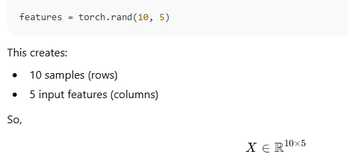
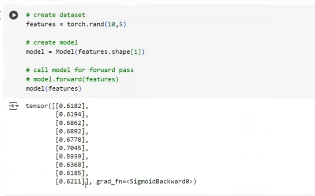
Dataset Creation

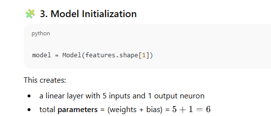
Model Initialization

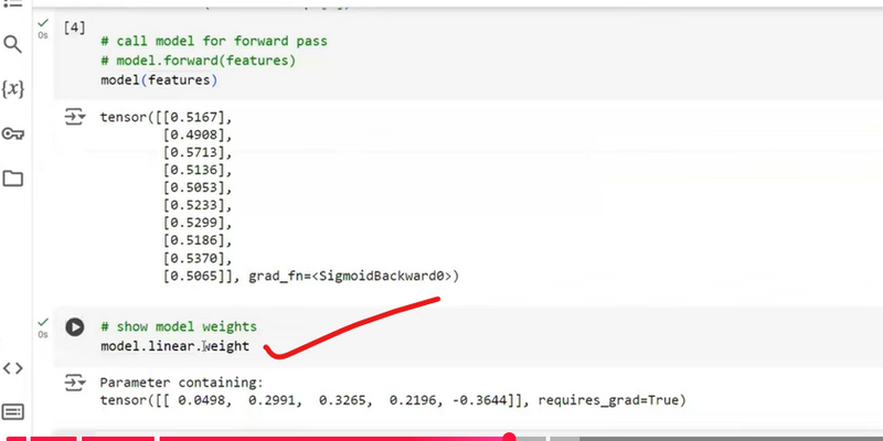
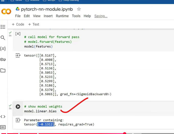
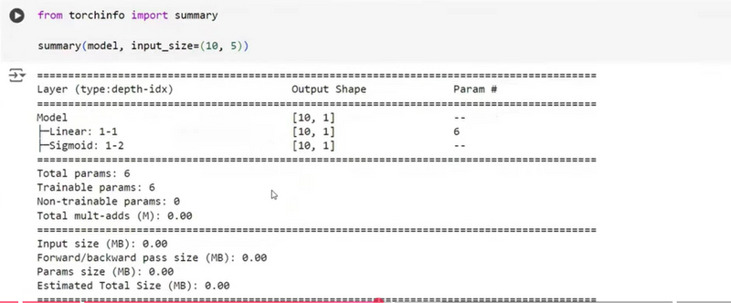
Comparsion of manual task and nn module with coding

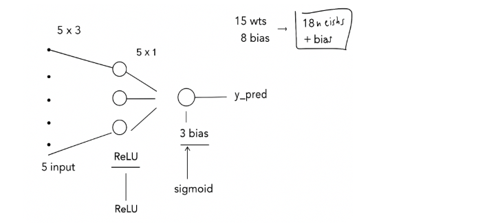
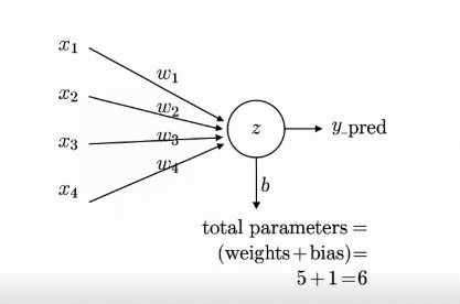
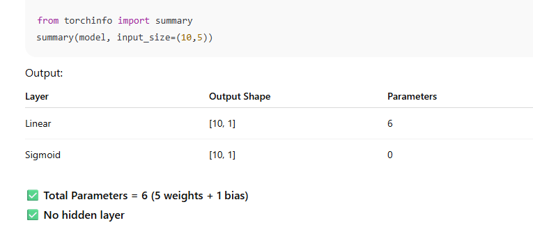
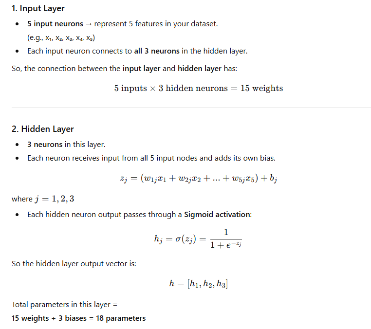
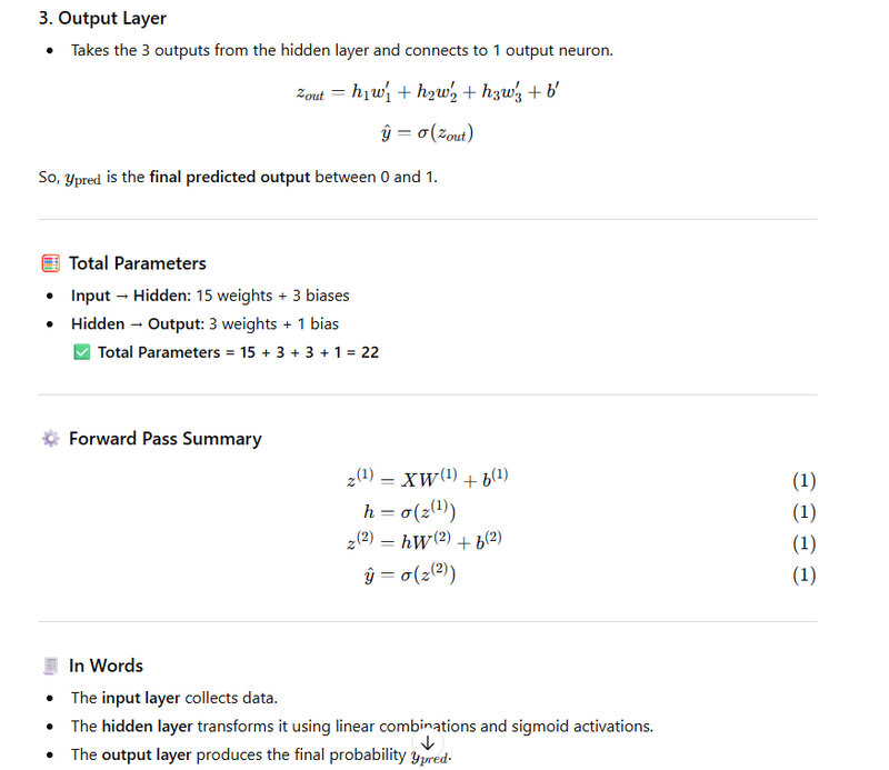
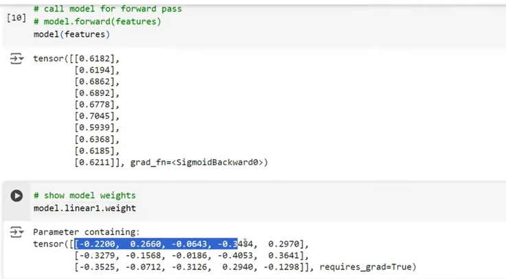
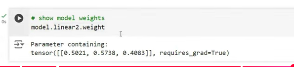
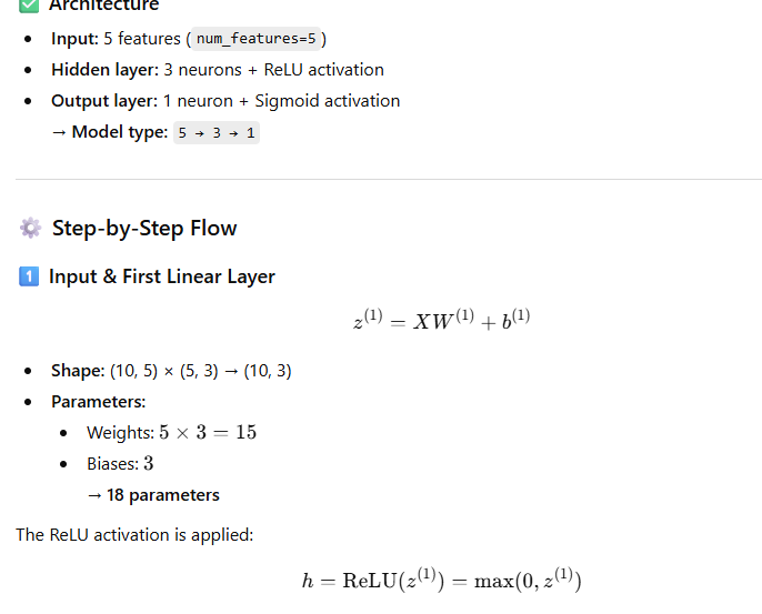
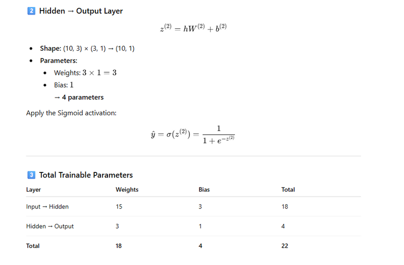
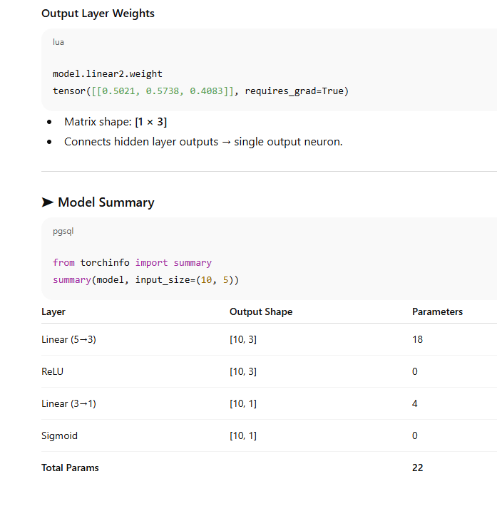
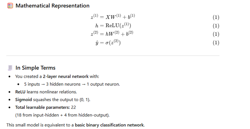
Neural Network Structure (5–3–1)

===============Or using sequential network==========

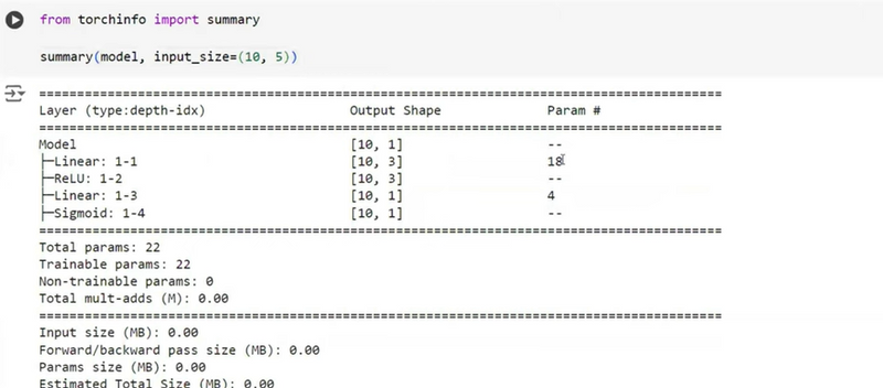
Explanation

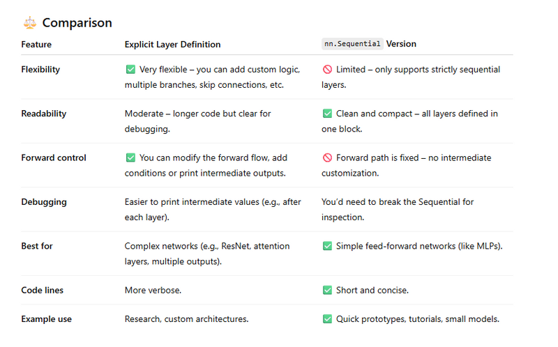
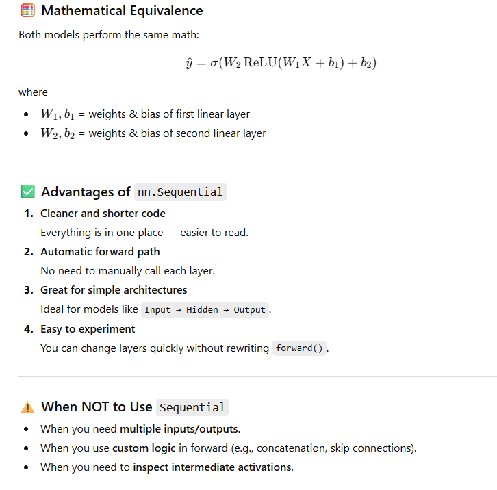
Advantage of nn.sequential netwok to create layers

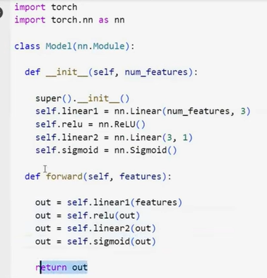
Traditional Explicit Definition

import torch
import torch.nn as nn

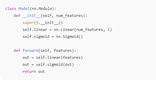
class Model(nn.Module):
    def __init__(self, num_features):
        super().__init__()
        self.linear1 = nn.Linear(num_features, 3)
        self.relu = nn.ReLU()
        self.linear2 = nn.Linear(3, 1)
        self.sigmoid = nn.Sigmoid()

    def forward(self, features):
        out = self.linear1(features)
        out = self.relu(out)
        out = self.linear2(out)
        out = self.sigmoid(out)
        return out

🔹 How it works

Each layer (linear1, relu, linear2, sigmoid) is created separately.

You explicitly define the forward path step-by-step.

Gives you fine control over every operation.

Using nn.Sequential

import torch
import torch.nn as nn

class Model(nn.Module):
    def __init__(self, num_features):
        super().__init__()
        self.network = nn.Sequential(
            nn.Linear(num_features, 3),
            nn.ReLU(),
            nn.Linear(3, 1),
            nn.Sigmoid()
        )

    def forward(self, features):
        return self.network(features)

🔹 How it works

nn.Sequential automatically chains all layers together.

The forward() pass executes all layers in the same order.

You only write the architecture once, not step-by-step.

How to use builtin loss and built in optimizer

How to use builtin loss and built in optimizer
How to use builtin loss and built in optimizer
Manual loss function

# define loss function
  def loss_function(self, y_pred, y):
    # Clamp predictions to avoid log(0)
    epsilon = 1e-7
    y_pred = torch.clamp(y_pred, epsilon, 1 - epsilon)

    # Calculate loss
    loss = -(y_train_tensor * torch.log(y_pred) + (1 - y_train_tensor) *       torch.log(1 - y_pred)).mean()
    return loss

  # loss calculate
  loss = model.loss_function(y_pred, y_train_tensor)

Built in loss function

# define loss function
loss_function = nn.BCELoss()

  # loss calculate
  loss = loss_function(y_pred, y_train_tensor.view(-1,1))

Manual optimizer

  # backward pass
  loss.backward()

  # parameters update
  with torch.no_grad():
    model.weights -= learning_rate * model.weights.grad
    model.bias -= learning_rate * model.bias.grad

  # zero gradients
  model.weights.grad.zero_()
  model.bias.grad.zero_()

Builtin optimizer

  # clear gradients
  optimizer.zero_grad()

  # backward pass
  loss.backward()

  # parameters update
  optimizer.step()

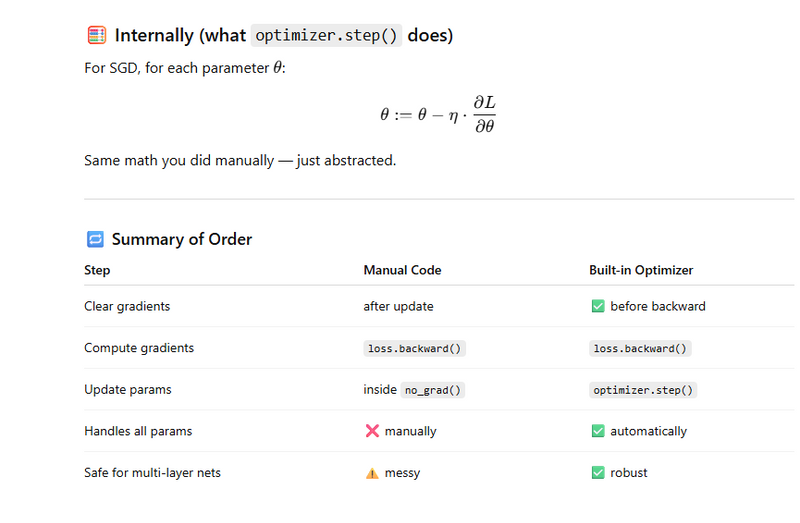
Differences between manual gradient descent and PyTorch’s built-in optimizers

*Your Manual Update Flow
*

# 1️⃣ backward pass
loss.backward()

# 2️⃣ parameter update
with torch.no_grad():
    model.weights -= learning_rate * model.weights.grad
    model.bias -= learning_rate * model.bias.grad

# 3️⃣ clear old gradients
model.weights.grad.zero_()
model.bias.grad.zero_()

🔍 What happens here

loss.backward() computes all gradients (∂L/∂W, ∂L/∂b).

You manually update weights and biases using the learning rate.

You then zero the gradients to prevent accumulation on the next iteration.

✅ Works fine for simple single-parameter models.

⚙️ Built-in Optimizer Flow (e.g., torch.optim.SGD, Adam, etc.)

# 1️⃣ clear gradients first
optimizer.zero_grad()

# 2️⃣ forward + loss
y_pred = model(X)
loss = criterion(y_pred, y)

# 3️⃣ backward pass
loss.backward()

# 4️⃣ update parameters
optimizer.step()

🔍 Why zero_grad() comes before backward

In PyTorch, gradients accumulate by default.

So before computing new gradients in this iteration, you clear the previous ones.

Otherwise, new grads would add on top of old grads, corrupting updates.

That’s why the order is:

zero_grad() → forward → loss → backward() → step()

This ensures:

Gradients from previous iteration are cleared.

New grads are computed via backpropagation.

Optimizer applies update to every parameter (weights + biases).

Everything stays in sync automatically.