Tensor flow basic operation
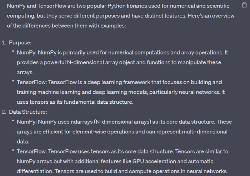
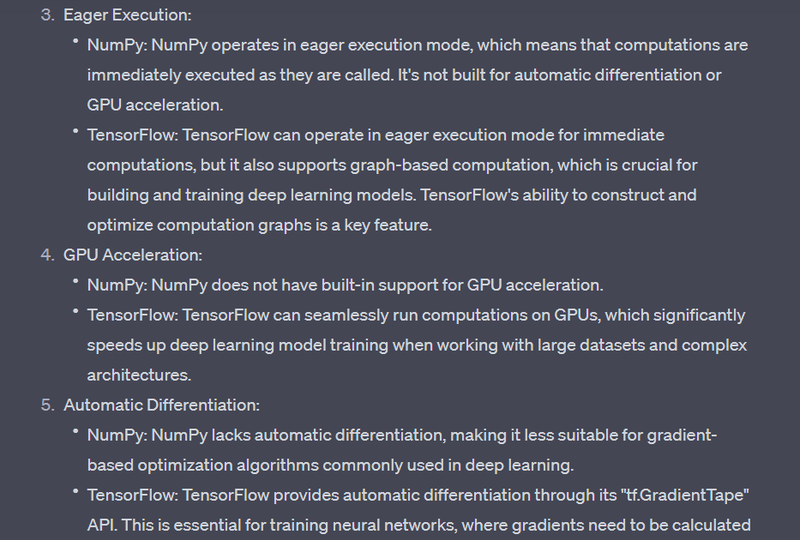
Difference between numpy and Tensor
Difference between numpy and Tensor and keras
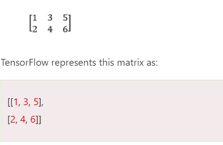
In TensorFlow, a tensor is the collection of feature vector (Like, array) of n-dimension. For instance, if we have any 2x3 matrix with values 1 to 6, we write:
Tensor flow basic operation
TensorFlow provides a wide range of operations (ops) for various machine learning and deep learning tasks. Here is a checklist of some common TensorFlow operations, along with examples and sample outputs:
Tensor Creation Ops:
tf.constant: Create a constant tensor.
a = tf.constant([1, 2, 3])
tf.Variable: Create a mutable variable tensor.
b = tf.Variable([4, 5, 6])
Math Ops:
tf.add, tf.subtract, tf.multiply, tf.divide: Perform element-wise arithmetic operations.
c = tf.add(a, b)  # Element-wise addition
d = tf.multiply(a, b)  # Element-wise multiplication
For example, if a is [1, 2, 3] and b is [4, 5, 6], then after performing the operations, you would get:

c will be [5, 7, 9] (element-wise addition).
d will be [4, 10, 18] (element-wise multiplication).
tf.matmul: Matrix multiplication.
e = tf.matmul(tf.constant([[1, 2], [3, 4]]), tf.constant([[5], [6]]))
Reduction Ops:
tf.reduce_mean, tf.reduce_sum: Compute the mean or sum of elements in a tensor.
mean_value = tf.reduce_mean(a)
sum_value = tf.reduce_sum(b)
Activation Functions:
tf.nn.relu, tf.nn.sigmoid, tf.nn.tanh, tf.nn.softmax: Common activation functions for neural networks.
output = tf.nn.relu(x)
Loss Functions:
tf.losses.mean_squared_error, tf.losses.softmax_cross_entropy: Common loss functions for training models.
loss = tf.losses.mean_squared_error(labels, predictions)

loss = tf.losses.softmax_cross_entropy(labels, predictions)
Optimization Ops:
tf.train.GradientDescentOptimizer, tf.train.AdamOptimizer: Create optimizers for gradient-based training.
optimizer = tf.train.AdamOptimizer(learning_rate=0.001)
Data Input Ops:
tf.data.Dataset: Create and manipulate datasets for input data.
dataset = tf.data.Dataset.from_tensor_slices(data)
Convolution Ops:
tf.nn.conv2d: Perform 2D convolution.
conv_output = tf.nn.conv2d(input, filters, strides=[1, 1, 1, 1], padding='SAME')
Pooling Ops:
tf.nn.max_pool: Perform max pooling.
pool_output = tf.nn.max_pool(input, ksize=[1, 2, 2, 1], strides=[1, 2, 2, 1], padding='SAME')
RNN Ops:
tf.keras.layers.SimpleRNN, tf.keras.layers.LSTM, tf.keras.layers.GRU: Create recurrent layers.
rnn_layer = tf.keras.layers.LSTM(units=64, return_sequences=True)(input_data)
Training Ops:
tf.GradientTape: Record gradients for automatic differentiation during training.
with tf.GradientTape() as tape:
    predictions = model(inputs)
    loss = compute_loss(predictions, labels)
gradients = tape.gradient(loss, model.trainable_variables)
Model Building Ops:
tf.keras.Sequential, tf.keras.Model: Build models using high-level APIs.
model = tf.keras.Sequential([
    tf.keras.layers.Dense(64, activation='relu'),
    tf.keras.layers.Dense(10, activation='softmax')
]).
Difference between numpy and Tensor
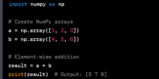
NumPy:
TensorFlow:
import tensorflow as tf

# Create TensorFlow tensors
a = tf.constant([1, 2, 3])
b = tf.constant([4, 5, 6])

# Element-wise addition
result = a + b
print(result)  # Output: [5 7 9]
Difference between numpy and Tensor and keras
NumPy:
NumPy is a fundamental package for scientific computing in Python. It provides support for large, multi-dimensional arrays and matrices, along with mathematical functions to operate on these arrays.
Example:
import numpy as np

# Create NumPy arrays
a = np.array([1, 2, 3])
b = np.array([4, 5, 6])

# Perform element-wise addition
c = a + b

# Print the result
print("NumPy Array Addition:", c)
Output:
NumPy Array Addition: [5 7 9]
TensorFlow:
TensorFlow is an open-source machine learning library developed by the Google Brain team. It is widely used for building and training deep learning models.
Example:
import tensorflow as tf

# Create TensorFlow tensors
a_tf = tf.constant([1, 2, 3], dtype=tf.float32)
b_tf = tf.constant([4, 5, 6], dtype=tf.float32)

# Perform element-wise addition using TensorFlow
c_tf = tf.add(a_tf, b_tf)

# Print the result
print("TensorFlow Tensor Addition:", c_tf.numpy())
Output:
TensorFlow Tensor Addition: [5. 7. 9.]
Keras (as part of TensorFlow):
Keras is a high-level neural networks API that runs on top of TensorFlow. It provides a user-friendly interface for building and training deep learning models.
Example:
from tensorflow.keras.models import Sequential
from tensorflow.keras.layers import Dense

# Create a Keras Sequential model
model = Sequential([
    Dense(units=3, activation='relu', input_shape=(3,)),
    Dense(units=1, activation='linear')
])

# Display the model architecture


model.summary()
Output:
Model: "sequential"
_________________________________________________________________
Layer (type)                 Output Shape              Param #
=================================================================
dense (Dense)                (None, 3)                 12
_________________________________________________________________
dense_1 (Dense)              (None, 1)                 4
=================================================================
Total params: 16
Trainable params: 16
Non-trainable params: 0
In this example, we create a simple Keras Sequential model with two dense layers.
In summary, NumPy is a general-purpose array-processing library, TensorFlow is a machine learning library that includes tools for deep learning, and Keras is a high-level neural networks API that runs on top of TensorFlow. They are often used together for building and training deep learning models. NumPy is more focused on array operations, while TensorFlow and Keras are specialized for machine learning tasks.
Eager Execution (TF 2.x default):
TensorFlow 2.x enables eager execution by default, making it easier to debug and understand the flow of your code.
tf.executing_eagerly() # Output: True
Explanation
The tf.executing_eagerly() function is used to check whether eager execution is enabled in TensorFlow. Eager execution allows operations to be executed immediately as they are called, which is useful for interactive development and debugging. It's the default mode in TensorFlow 2.x, but in TensorFlow 1.x, you might need to enable it explicitly.
Here's an example of how and when to use tf.executing_eagerly()
import tensorflow as tf

# Check if eager execution is enabled
print("Eager execution is enabled: ", tf.executing_eagerly())

# Enable eager execution (not necessary in TensorFlow 2.x)
tf.compat.v1.enable_eager_execution()

# Check again after enabling eager execution
print("Eager execution is enabled: ", tf.executing_eagerly())

# Simple computation with tensors
a = tf.constant(2)
b = tf.constant(3)
c = a + b

# Print the result
print("Sum of a and b: ", c.numpy())
Output
Eager execution is enabled:  True
Eager execution is enabled:  True
Sum of a and b:  5
Check if Eager Execution is Enabled:
The first line prints the current status of eager execution. In TensorFlow 2.x, it's enabled by default. In TensorFlow 1.x, you may need to enable it using tf.compat.v1.enable_eager_execution().
Enable Eager Execution (If Necessary):
If you're using TensorFlow 1.x, you might need to enable eager execution explicitly using tf.compat.v1.enable_eager_execution(). In TensorFlow 2.x, this is not necessary.
Check Again:
After enabling eager execution, the second print statement confirms that it's indeed enabled.
Simple Computation:
The code performs a simple computation using TensorFlow constants. Since eager execution is enabled, the result is immediately available, and you can access it using the numpy() method.
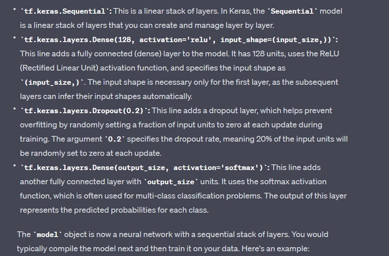
Create a Model (Sequential API):
model = tf.keras.Sequential([
    tf.keras.layers.Dense(128, activation='relu', input_shape=(input_size,)),
    tf.keras.layers.Dropout(0.2),
    tf.keras.layers.Dense(output_size, activation='softmax')
])
Define a Placeholder (In TensorFlow 1.x):
TensorFlow 2.x doesn't use placeholders in eager execution mode. However, if you still want to use placeholders, you can do so in
x = tf.placeholder(tf.float32, shape=(None, input_size))
Explanation
tf.placeholder(tf.float32, shape=(None, input_size)): This line creates a placeholder tensor named x. A placeholder is a symbolic variable that is used as the input to the computational graph. In this case, it's a 2D tensor of type float32 with a variable number of rows (None) and input_size columns. The None dimension allows for a variable batch size, meaning you can feed in different-sized batches of data during runtime.
If you were to use this placeholder in a TensorFlow 1.x session, you would typically provide a feed_dict to pass actual values during execution. Here's a simple example:
import tensorflow as tf

# Assume input_size is defined earlier

# Create a placeholder
x = tf.placeholder(tf.float32, shape=(None, input_size))

# Define an operation
y = tf.square(x)

# Create a session
with tf.Session() as sess:
    # Feed actual data to the placeholder
    input_data = [[1.0, 2.0, 3.0], [4.0, 5.0, 6.0]]
    result = sess.run(y, feed_dict={x: input_data})

# Output the result
print(result)
Another Example
input_size = 784  # Assuming a specific input size
x = tf.placeholder(tf.float32, shape=(None, input_size))

W = tf.Variable(tf.zeros([input_size, 10]))
b = tf.Variable(tf.zeros([10]))
logits = tf.matmul(x, W) + b
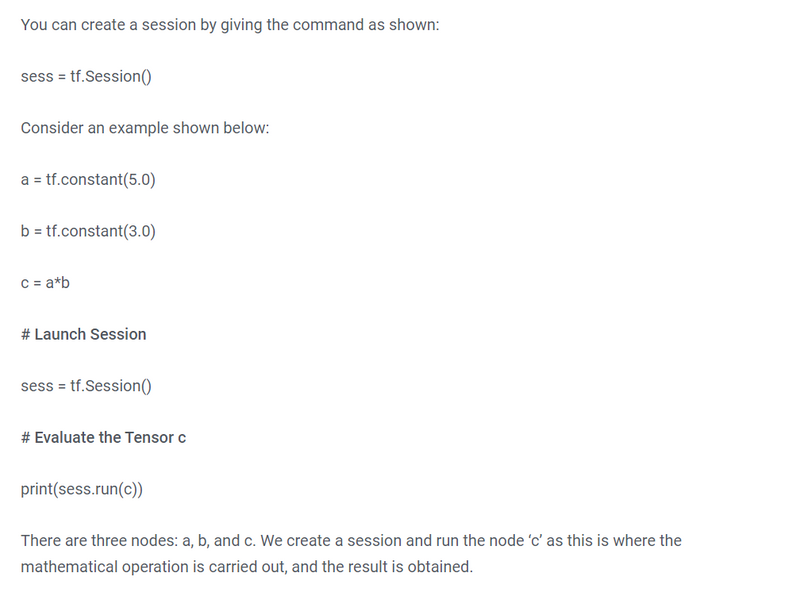
Session (In TensorFlow 1.x):
TensorFlow 2.x does not require explicit session management due to eager execution. However, for TensorFlow 1.x, you might need to use sessions.
with tf.Session() as sess:
    result = sess.run(some_operation)
with tf.Session() as sess:: This line creates a TensorFlow session using a context manager (with statement). The session is responsible for executing operations in a TensorFlow graph.
result = sess.run(some_operation): Inside the session block, this line runs the operation some_operation using the run method of the session. The run method is used to execute operations in the graph and fetch the results.
Now, let's consider a more concrete example to illustrate the usage:
import tensorflow as tf

# Define a simple operation
a = tf.constant(3)
b = tf.constant(4)
some_operation = a + b

# Execute the operation within a session
with tf.Session() as sess:
    result = sess.run(some_operation)

# Output the result
print(result)
Output:
7
Feed Data Using feed_dict (In TensorFlow 1.x):
with tf.Session() as sess:
    result = sess.run(some_operation, feed_dict={x: input_data})
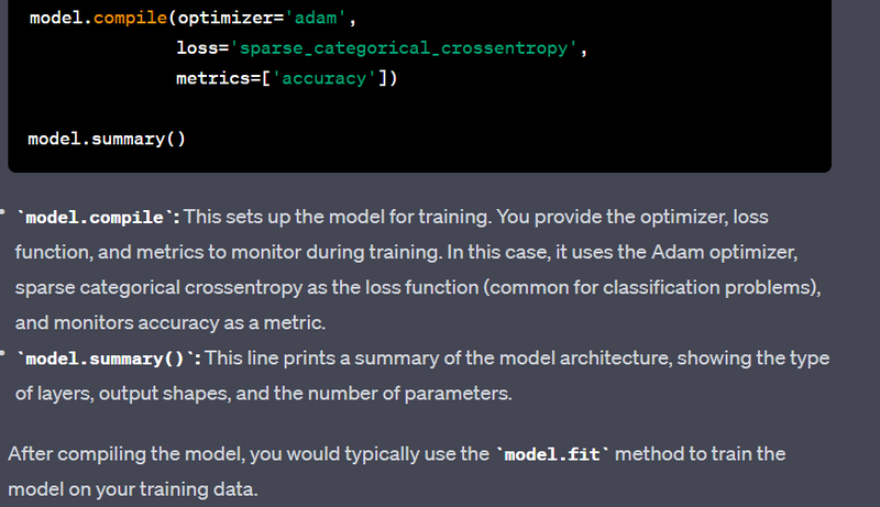
Model Training:
model.compile(optimizer='adam',
              loss='sparse_categorical_crossentropy',
              metrics=['accuracy'])

model.fit(x_train, y_train, epochs=5)
Save and Load the Model:
model.save('my_model.h5')
loaded_model = tf.keras.models.load_model('my_model.h5')
TensorBoard (Optional for Visualization):
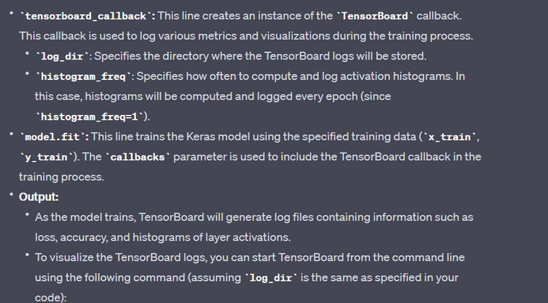
tensorboard_callback = tf.keras.callbacks.TensorBoard(log_dir=log_dir, histogram_freq=1)
model.fit(x_train, y_train, epochs=5, callbacks=[tensorboard_callback])
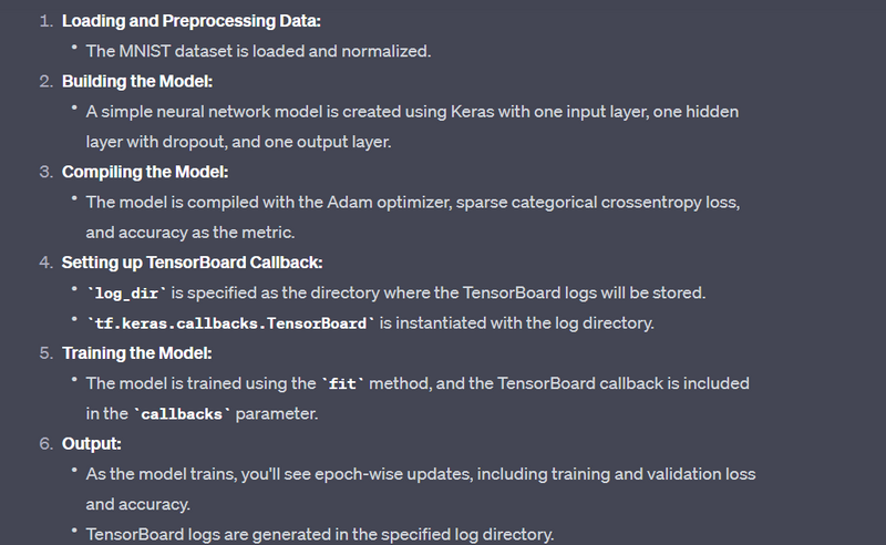
import tensorflow as tf
from tensorflow.keras import layers, models
from tensorflow.keras.datasets import mnist

# Load and preprocess the data
(x_train, y_train), (x_test, y_test) = mnist.load_data()
x_train, x_test = x_train / 255.0, x_test / 255.0

# Build a simple neural network model
model = models.Sequential([
    layers.Flatten(input_shape=(28, 28)),
    layers.Dense(128, activation='relu'),
    layers.Dropout(0.2),
    layers.Dense(10, activation='softmax')
])

# Compile the model
model.compile(optimizer='adam',
              loss='sparse_categorical_crossentropy',
              metrics=['accuracy'])

# Specify the log directory for TensorBoard
log_dir = "logs/fit/"
tensorboard_callback = tf.keras.callbacks.TensorBoard(log_dir=log_dir, histogram_freq=1)

# Train the model with the TensorBoard callback
model.fit(x_train, y_train, epochs=5, validation_data=(x_test, y_test), callbacks=[tensorboard_callback])
Visualizing in TensorBoard:
Start TensorBoard from the command line:
tensorboard --logdir=logs/fit/
Open a web browser and navigate to the specified port (usually http://localhost:6006).
In TensorBoard, you can explore various tabs such as Scalars, Graphs, and Histograms.
This example demonstrates how to use TensorBoard to visualize and monitor the training process, making it easier to understand model performance, identify issues, and optimize your neural network.


Top comments (0)