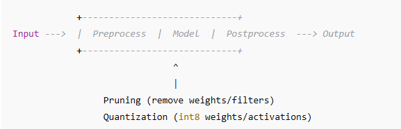
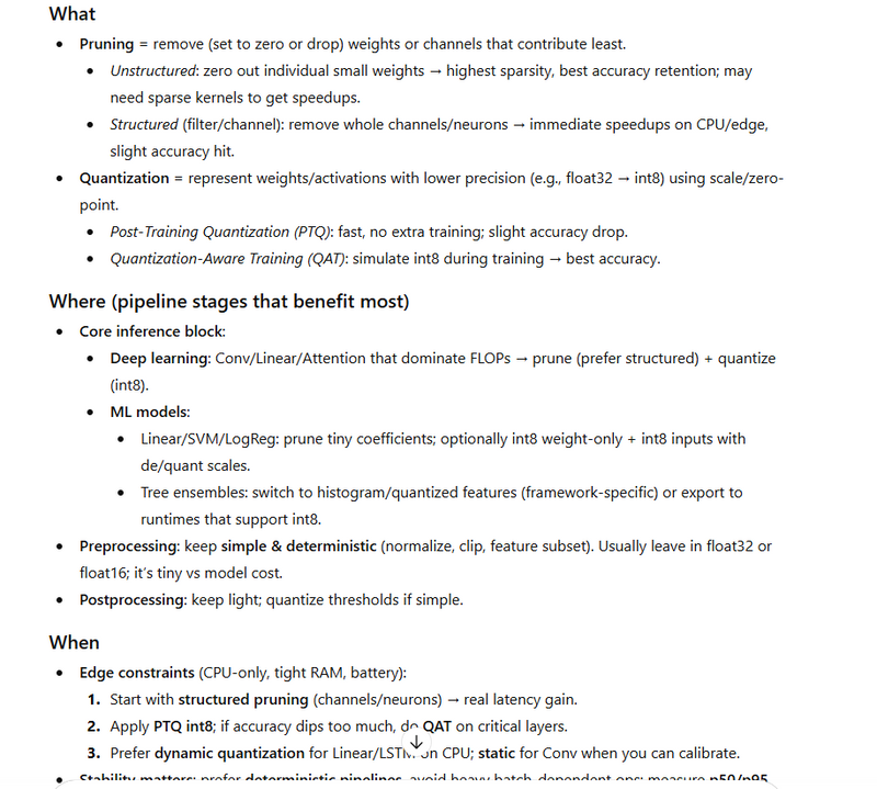
Pruning
= delete (or zero-out) parts of a model that contribute little → fewer FLOPs, fewer parameters, faster inference.
Quantization
= store & compute with fewer bits (e.g., 8-bit instead of 32-bit floats) → smaller memory, higher cache hits, faster CPU ops.
Both aim to fit tight edge budgets (CPU-only, small RAM) while keeping accuracy good enough for real-time control.
Where they act in a network
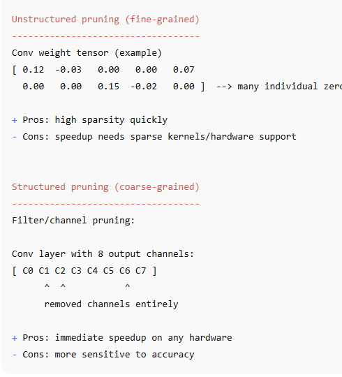
Two flavors of pruning
Quantization pipeline (typical PTQ)
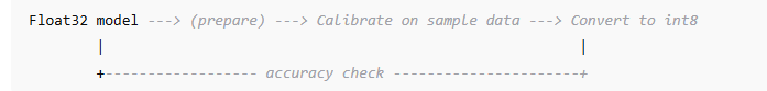
PTQ (Post-Training Quantization): No training required. Fastest path to int8.
QAT (Quantization-Aware Training): Train with fake-quant modules → better accuracy at int8, especially for CNNs.
Why robots care
Latency (ms-level) & consistency (low jitter) matter for control loops.
Size matters (RAM/flash budgets).
Robustness to noise: simpler models + calibrated quantization + structured pruning → fewer surprises.
Metrics to watch
Accuracy (task metric)
Latency (avg & p95/p99)
Model size (MB)
Sparsity (% zeros) & MACs/FLOPs
Energy (optional but relevant on battery)
ML EXAMPLES (scikit-learn)
We’ll show:
Decision Tree pruning (cost-complexity)
L1 “pruning” of linear/logistic models (drives coefficients to zero)
Note: Classic scikit-learn doesn’t do int8 quantization of models end-to-end; for edge you often export to ONNX + use runtimes that quantize, or you choose small models + pruning/L1.
1) Decision Tree – cost-complexity pruning
# ml_pruning_tree.py
import time
import numpy as np
from sklearn.datasets import load_iris
from sklearn.model_selection import train_test_split
from sklearn.tree import DecisionTreeClassifier
from sklearn.tree import plot_tree  # optional (for visualization)
from sklearn.metrics import accuracy_score

X, y = load_iris(return_X_y=True)
Xtr, Xte, ytr, yte = train_test_split(X, y, test_size=0.2, random_state=42)

# Baseline (unpruned)
base = DecisionTreeClassifier(random_state=42)
base.fit(Xtr, ytr)

# Cost complexity pruning path gives candidate ccp_alphas
path = base.cost_complexity_pruning_path(Xtr, ytr)
ccp_alphas = path.ccp_alphas

best = None
best_stats = None

for ccp in ccp_alphas:
    clf = DecisionTreeClassifier(random_state=42, ccp_alpha=ccp)
    clf.fit(Xtr, ytr)
    # measure latency per sample (simple timing)
    t0 = time.time()
    ypred = clf.predict(Xte)
    t1 = time.time()
    acc = accuracy_score(yte, ypred)
    latency_ms = (t1 - t0) / len(Xte) * 1000.0
    n_nodes = clf.tree_.node_count
    stats = (acc, latency_ms, n_nodes, ccp)
    if best is None or (acc > best_stats[0]) or (acc == best_stats[0] and latency_ms < best_stats[1]):
        best, best_stats = clf, stats

print(f"Best pruned tree:")
print(f"  accuracy = {best_stats[0]:.3f}")
print(f"  latency  = {best_stats[1]:.3f} ms/sample")
print(f"  nodes    = {best_stats[2]} (ccp_alpha={best_stats[3]:.6f})")


What this gives: a smaller tree → fewer branches → faster, more stable inference on CPU.
2) L1 “pruning” (sparse coefficients)
# ml_pruning_l1.py
import time
import numpy as np
from sklearn.datasets import load_iris
from sklearn.model_selection import train_test_split
from sklearn.linear_model import LogisticRegression
from sklearn.metrics import accuracy_score

X, y = load_iris(return_X_y=True)
Xtr, Xte, ytr, yte = train_test_split(X, y, test_size=0.2, random_state=42)

# L1 penalty drives many weights to zero (like pruning)
clf = LogisticRegression(penalty='l1', solver='saga', C=0.5, max_iter=500, multi_class='auto')
clf.fit(Xtr, ytr)

t0 = time.time()
yp = clf.predict(Xte)
t1 = time.time()

acc = accuracy_score(yte, yp)
latency_ms = (t1 - t0) / len(Xte) * 1000.0
sparsity = np.mean(clf.coef_ == 0.0)

print(f"Accuracy      : {acc:.3f}")
print(f"Latency       : {latency_ms:.3f} ms/sample")
print(f"Weight zeros  : {sparsity*100:.1f}%")
Takeaway: Smaller effective feature set → cache-friendly, consistent latency.
DL EXAMPLES (PyTorch)
We’ll show:
Unstructured & structured pruning via torch.nn.utils.prune
Dynamic PTQ (int8) for Linear/LSTM
Static PTQ (FX graph mode) for a tiny CNN (with calibration)
QAT sketch for best accuracy at int8
These run on CPU and illustrate what to change. Replace synthetic data with your sensor features.
Helper: latency + size + sparsity utilities
# utils_perf.py
import time
import torch
import os

def measure_latency_ms(model, inp, n_warm=10, n_runs=50):
    model.eval()
    with torch.no_grad():
        for _ in range(n_warm):
            _ = model(inp)
        t0 = time.time()
        for _ in range(n_runs):
            _ = model(inp)
        t1 = time.time()
    return (t1 - t0) / n_runs * 1000.0

def count_nonzero_params(model):
    nz = 0
    tot = 0
    for p in model.parameters():
        tot += p.numel()
        nz += (p != 0).sum().item()
    return nz, tot, 1.0 - nz / tot

def save_size_mb(model, path="temp.pth"):
    torch.save(model.state_dict(), path)
    sz = os.path.getsize(path) / (1024*1024)
    os.remove(path)
    return sz
A. PRUNING (PyTorch)
A1) Unstructured pruning (magnitude)
# dl_prune_unstructured.py
import torch
import torch.nn as nn
import torch.nn.utils.prune as prune
from utils_perf import measure_latency_ms, count_nonzero_params, save_size_mb

# Tiny MLP for demonstration
class MLP(nn.Module):
    def __init__(self, d_in=64, d_hidden=128, d_out=10):
        super().__init__()
        self.net = nn.Sequential(
            nn.Linear(d_in, d_hidden),
            nn.ReLU(),
            nn.Linear(d_hidden, d_out)
        )
    def forward(self, x):
        return self.net(x)

model = MLP()
inp = torch.randn(1, 64)

lat0 = measure_latency_ms(model, inp)
nz0, tot0, sparsity0 = count_nonzero_params(model)
size0 = save_size_mb(model)

# Apply 80% unstructured pruning on Linear weights
for m in model.modules():
    if isinstance(m, nn.Linear):
        prune.l1_unstructured(m, name="weight", amount=0.8)

# Remove reparametrization (make pruning permanent)
for m in model.modules():
    if isinstance(m, nn.Linear) and hasattr(m, "weight_orig"):
        prune.remove(m, "weight")

lat1 = measure_latency_ms(model, inp)
nz1, tot1, sparsity1 = count_nonzero_params(model)
size1 = save_size_mb(model)

print(f"Latency (ms)   before/after: {lat0:.3f} / {lat1:.3f}")
print(f"Sparsity       before/after: {sparsity0*100:.1f}% / {sparsity1*100:.1f}%")
print(f"Model size (MB)before/after: {size0:.3f} / {size1:.3f}")
Note: Unstructured zeros may not speed up on vanilla kernels; you get memory benefits and speedups only if using sparse backends. For deterministic speed on CPU, prefer structured pruning.
A2) Structured channel pruning (conv channels)
# dl_prune_structured.py
import torch
import torch.nn as nn
import torch.nn.utils.prune as prune
from utils_perf import measure_latency_ms, count_nonzero_params, save_size_mb

class TinyCNN(nn.Module):
    def __init__(self):
        super().__init__()
        self.conv1 = nn.Conv2d(3, 16, 3, padding=1)
        self.relu = nn.ReLU()
        self.conv2 = nn.Conv2d(16, 32, 3, padding=1)
        self.pool = nn.AdaptiveAvgPool2d(1)
        self.fc = nn.Linear(32, 10)
    def forward(self, x):
        x = self.relu(self.conv1(x))
        x = self.relu(self.conv2(x))
        x = self.pool(x).flatten(1)
        return self.fc(x)

model = TinyCNN()
inp = torch.randn(1, 3, 64, 64)

lat0 = measure_latency_ms(model, inp)
nz0, tot0, s0 = count_nonzero_params(model)
size0 = save_size_mb(model)

# Prune entire output channels from conv2 (e.g., 50%)
# amount is fraction of channels to remove; dim=0 means output channels
prune.ln_structured(model.conv2, name="weight", amount=0.5, n=2, dim=0)
prune.remove(model.conv2, "weight")

lat1 = measure_latency_ms(model, inp)
nz1, tot1, s1 = count_nonzero_params(model)
size1 = save_size_mb(model)

print(f"Latency (ms)   before/after: {lat0:.3f} / {lat1:.3f}")
print(f"Sparsity       before/after: {s0*100:.1f}% / {s1*100:.1f}%")
print(f"Model size (MB)before/after: {size0:.3f} / {size1:.3f}")
Why structured helps: removed channels shrink subsequent ops → actual FLOP reduction and stable CPU speedups.
B. QUANTIZATION (PyTorch)
B1) Dynamic quantization (fastest path; great for Linear/LSTM on CPU)
# dl_quant_dynamic.py
import torch
import torch.nn as nn
from utils_perf import measure_latency_ms, save_size_mb

class TinyRNN(nn.Module):
    def __init__(self, d_in=32, d_hidden=64, d_out=6):
        super().__init__()
        self.rnn = nn.LSTM(d_in, d_hidden, num_layers=1, batch_first=True)
        self.fc = nn.Linear(d_hidden, d_out)
    def forward(self, x):
        # x: [B, T, d_in]
        y, _ = self.rnn(x)
        return self.fc(y[:, -1, :])

model_fp32 = TinyRNN().eval()
inp = torch.randn(1, 20, 32)

lat0 = measure_latency_ms(model_fp32, inp)
size0 = save_size_mb(model_fp32)

# Dynamic quantize only supported layer types (Linear, LSTM)
model_int8 = torch.ao.quantization.quantize_dynamic(
    model_fp32, {nn.Linear, nn.LSTM}, dtype=torch.qint8
).eval()

lat1 = measure_latency_ms(model_int8, inp)
size1 = save_size_mb(model_int8)

print(f"Latency (ms)   FP32 / INT8(dynamic): {lat0:.3f} / {lat1:.3f}")
print(f"Model size (MB)FP32 / INT8(dynamic): {size0:.3f} / {size1:.3f}")
Use when: CPU edge device, MLP/RNN control heads, quick wins without retraining.
B2) Static PTQ (FX graph mode) for a tiny CNN
# dl_quant_static_ptq.py
import torch
import torch.nn as nn
from torch.ao.quantization import get_default_qconfig_mapping
from torch.ao.quantization.quantize_fx import prepare_fx, convert_fx
from utils_perf import measure_latency_ms, save_size_mb

class TinyCNN(nn.Module):
    def __init__(self):
        super().__init__()
        self.seq = nn.Sequential(
            nn.Conv2d(3, 16, 3, stride=1, padding=1),
            nn.ReLU(),
            nn.Conv2d(16, 16, 3, stride=1, padding=1),
            nn.ReLU(),
            nn.AdaptiveAvgPool2d(1),
            nn.Flatten(),
            nn.Linear(16, 10)
        )
    def forward(self, x):
        return self.seq(x)

model = TinyCNN().eval()
example = torch.randn(1, 3, 64, 64)

lat0 = measure_latency_ms(model, example)
size0 = save_size_mb(model)

# 1) Choose backend/qconfig
backend = "qnnpack"  # good for ARM/Android; "fbgemm" for x86
torch.backends.quantized.engine = backend
qconfig_mapping = get_default_qconfig_mapping(backend)

# 2) Prepare FX graph
prepared = prepare_fx(model, {"": qconfig_mapping})

# 3) Calibrate with a small representative set
prepared(torch.randn(1,3,64,64))
prepared(torch.randn(1,3,64,64))
prepared(torch.randn(1,3,64,64))

# 4) Convert to int8
int8_model = convert_fx(prepared).eval()

lat1 = measure_latency_ms(int8_model, example)
size1 = save_size_mb(int8_model)

print(f"Latency (ms)   FP32 / INT8(static): {lat0:.3f} / {lat1:.3f}")
print(f"Model size (MB)FP32 / INT8(static): {size0:.3f} / {size1:.3f}")
Calibrate carefully: use a few hundred real sensor samples for best accuracy.
B3) QAT sketch (best accuracy @ int8 for CNNs)
# dl_qat_skeleton.py
import torch
import torch.nn as nn
import torch.optim as optim
from torch.ao.quantization import get_default_qat_qconfig_mapping
from torch.ao.quantization.quantize_fx import prepare_qat_fx, convert_fx

class TinyCNN(nn.Module):
    def __init__(self):
        super().__init__()
        self.seq = nn.Sequential(
            nn.Conv2d(3, 16, 3, padding=1), nn.ReLU(),
            nn.Conv2d(16,16,3,padding=1),   nn.ReLU(),
            nn.AdaptiveAvgPool2d(1), nn.Flatten(), nn.Linear(16, 10)
        )
    def forward(self, x): return self.seq(x)

model = TinyCNN().train()
backend = "qnnpack"
torch.backends.quantized.engine = backend
qconfig_mapping = get_default_qat_qconfig_mapping(backend)

# Insert fake-quant observers
model_qat = prepare_qat_fx(model, {"": qconfig_mapping}).train()

opt = optim.Adam(model_qat.parameters(), lr=1e-3)

# Train as usual (fake-quant active)
for step in range(200):  # demo loop
    x = torch.randn(16,3,64,64)
    y = torch.randint(0,10,(16,))
    logits = model_qat(x)
    loss = nn.CrossEntropyLoss()(logits, y)
    opt.zero_grad(); loss.backward(); opt.step()

# Convert to real int8
model_int8 = convert_fx(model_qat.eval()).eval()
Putting it together: which stages benefit most?
Perception & control networks (Conv/MLP/RNN heads) → Quantization (int8) + Structured pruning (channels) for real CPU gains.
Feature encoders (heavy backbones) → QAT (keep accuracy) + careful structured pruning of later blocks.
Classical ML pieces (trees, linear heads) → prune (cost-complexity / L1) and/or replace with smaller models; quantization usually handled by deployment runtime if needed.
Practical workflow (ASCII diagram)
Train FP32  --->  Profile (lat/size/acc)  --->  Choose targets
                                         \
                                          \--> Structured prune (channels/heads) -> Fine-tune
                                              -> PTQ (dynamic/static) or QAT
                                              -> Re-profile (p50/p95 latency, acc, size)
                                              -> Iterate until SLA met
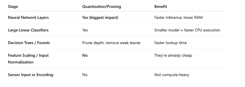
Which Stages Benefit Most from Quantization or Pruning?
Best Stage to Apply Quantization/Pruning
The Model / Inference Stage
This is where matrix multiplications and decision logic happen.
❌ Not Useful to Quantize/Prune
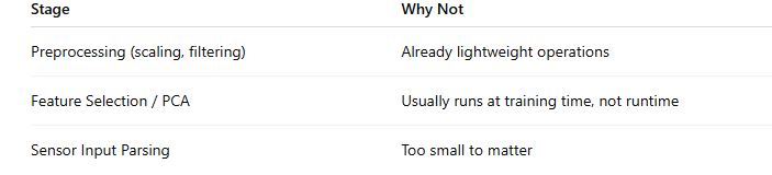
So:
The parts that benefit the most are:
Neural network layers (Linear, Conv, GRU/LSTM)
Decision trees / Random Forests (by pruning depth or removing weak nodes)
Large linear models (by pruning small-magnitude weights)
Part 1: Classical ML Example
We will:
Train Logistic Regression
Prune small weights
Quantize model weights to float16 to reduce memory + improve speed
# ===== classical_prune_quant.py =====
import numpy as np
from sklearn.datasets import load_iris
from sklearn.preprocessing import StandardScaler
from sklearn.linear_model import LogisticRegression
from sklearn.pipeline import Pipeline
from sklearn.metrics import accuracy_score

# Load dataset
data = load_iris()
X, y = data.data, data.target

# Build pipeline
pipe = Pipeline([
    ("scaler", StandardScaler()),
    ("clf", LogisticRegression(max_iter=500, multi_class='multinomial'))
])

pipe.fit(X, y)
clf = pipe.named_steps["clf"]

print("Original weights shape:", clf.coef_.shape)

# ----- PRUNING: remove small weights -----
threshold = np.percentile(np.abs(clf.coef_), 20)   # prune 20% smallest weights
mask = np.abs(clf.coef_) > threshold
clf.coef_ = clf.coef_ * mask

print("Pruned weights mean magnitude:", np.mean(np.abs(clf.coef_)))

# ----- QUANTIZATION: convert to float16 -----
clf.coef_  = clf.coef_.astype(np.float16)
clf.intercept_ = clf.intercept_.astype(np.float16)

print("After quantization dtype:", clf.coef_.dtype)

# Check accuracy
y_pred = pipe.predict(X)
print("Accuracy after prune + quant:", accuracy_score(y, y_pred))
Result:
Model is lighter, smaller, and usually faster on edge CPUs.
Accuracy remains similar (because small weights typically don’t matter).
✅
Part 2: Deep Learning Example (PyTorch)
We will:
Train a tiny MLP
Prune weights with torch.nn.utils.prune
Quantize using PyTorch dynamic quantization
Compare latency
# ===== dl_prune_quant.py =====
import torch
import torch.nn as nn
import torch.nn.utils.prune as prune
import time
import numpy as np

# Create dummy dataset
X = torch.randn(300, 16)
y = torch.randint(0, 3, (300,))

# Tiny MLP model
class MLP(nn.Module):
    def __init__(self):
        super().__init__()
        self.fc1 = nn.Linear(16, 32)
        self.fc2 = nn.Linear(32, 3)
    def forward(self, x):
        return self.fc2(torch.relu(self.fc1(x)))

model = MLP()
criterion = nn.CrossEntropyLoss()
optimizer = torch.optim.Adam(model.parameters(), lr=1e-2)

# Train briefly
for _ in range(200):
    optimizer.zero_grad()
    loss = criterion(model(X), y)
    loss.backward()
    optimizer.step()

# -------- PRUNING --------
prune.l1_unstructured(model.fc1, name="weight", amount=0.3)  # prune 30% of weights
prune.remove(model.fc1, 'weight')  # finalize mask

# -------- QUANTIZATION --------
quantized_model = torch.quantization.quantize_dynamic(
    model, {nn.Linear}, dtype=torch.qint8
)

# -------- LATENCY TEST --------
def bench(model):
    model.eval()
    times=[]
    for _ in range(500):
        inp = torch.randn(1,16)
        t0=time.time()
        _=model(inp)
        times.append((time.time()-t0)*1000)
    return np.mean(times), np.percentile(times,95)

fp32_mean, fp32_p95 = bench(model)
int8_mean, int8_p95 = bench(quantized_model)

print("FP32 latency avg:", fp32_mean, "ms  p95:", fp32_p95)
print("INT8 latency avg:", int8_mean, "ms  p95:", int8_p95)
Full Code — ML (scikit-learn + NumPy int8)
This example shows:
Train a Logistic Regression on the digits dataset.
Prune small coefficients by magnitude.
Quantize weights and inputs to int8 with scale/zero-point.
Evaluate accuracy and average latency.
# ===== ML PRUNING + INT8 QUANTIZATION (SCIKIT + NUMPY) =====
import numpy as np
import time
from sklearn.datasets import load_digits
from sklearn.model_selection import train_test_split
from sklearn.preprocessing import StandardScaler
from sklearn.linear_model import LogisticRegression
from sklearn.metrics import accuracy_score

# --- Data ---
digits = load_digits()
X = digits.data.astype(np.float32)  # shape (n, 64)
y = digits.target
X_train, X_test, y_train, y_test = train_test_split(X, y, test_size=0.2, random_state=42, stratify=y)

# Standardize inputs (stable normalization for noisy sensors)
scaler = StandardScaler()
X_train = scaler.fit_transform(X_train)
X_test  = scaler.transform(X_test)

# --- Baseline model ---
clf = LogisticRegression(max_iter=200, solver="saga", penalty="l2", n_jobs=-1)
clf.fit(X_train, y_train)
base_pred = clf.predict(X_test)
base_acc = accuracy_score(y_test, base_pred)

# --- PRUNING: zero out small coefficients by magnitude ---
def prune_coef(clf, sparsity=0.3):
    # sparsity = fraction of weights to zero by magnitude (per class)
    W = clf.coef_.copy()  # [n_classes, n_features]
    B = clf.intercept_.copy()

    pruned_W = W.copy()
    for c in range(W.shape[0]):
        w = W[c]
        k = int(np.floor(sparsity * w.size))
        if k <= 0:
            continue
        thresh = np.partition(np.abs(w), k)[k]
        mask = np.abs(w) >= thresh
        pruned_W[c] = w * mask  # zero-out small weights

    return pruned_W, B

pruned_W, pruned_B = prune_coef(clf, sparsity=0.3)

# --- QUANTIZATION: per-tensor int8 for weights and inputs ---
# Helper: affine quantization (symmetric zero-point for simplicity)
def quantize_per_tensor(x, num_bits=8):
    qmin, qmax = -128, 127
    max_abs = np.max(np.abs(x)) + 1e-8
    scale = max_abs / qmax
    zp = 0
    x_q = np.clip(np.round(x / scale), qmin, qmax).astype(np.int8)
    return x_q, scale, zp

def dequantize_per_tensor(x_q, scale, zp=0):
    return (x_q.astype(np.float32) - zp) * scale

# Quantize weights (one scale per class to keep it simple)
W_q_list, W_scales = [], []
for c in range(pruned_W.shape[0]):
    W_q, s, _ = quantize_per_tensor(pruned_W[c])
    W_q_list.append(W_q)
    W_scales.append(s)
W_q = np.stack(W_q_list, axis=0).astype(np.int8)   # [C, F]
W_scales = np.array(W_scales, dtype=np.float32)    # [C]
B_q, B_scale, _ = quantize_per_tensor(pruned_B)    # bias int8; small accuracy hit but shows the idea

# Quantize inputs with a single global scale (simple & fast)
X_scale = np.max(np.abs(X_train)) / 127.0 + 1e-8

def predict_int8(Xf):
    # Quantize input
    X_q = np.clip(np.round(Xf / X_scale), -128, 127).astype(np.int8)  # [N, F]

    # Matmul in int32: logits_q = W_q @ X_q.T + B_q
    # We'll dequantize to float for soft argmax (largest logit).
    # Effective scale per class = (W_scale[c] * X_scale)
    logits = []
    X_q_T = X_q.T.astype(np.int32)  # [F, N]
    for c in range(W_q.shape[0]):
        # int8 dot → int32
        dot_int32 = (W_q[c].astype(np.int32) @ X_q_T)  # [N]
        # dequantize weights*inputs
        fl = dot_int32.astype(np.float32) * (W_scales[c] * X_scale)
        # add (dequantized) bias
        fl += dequantize_per_tensor(B_q[c], B_scale)
        logits.append(fl)
    logits = np.stack(logits, axis=1)  # [N, C]
    return np.argmax(logits, axis=1)

# --- Evaluate accuracy and latency ---
start = time.time()
y_pred_int8 = predict_int8(X_test)
lat = (time.time() - start) / len(X_test) * 1000.0  # ms/sample

int8_acc = accuracy_score(y_test, y_pred_int8)

print(f"Baseline float32 Accuracy: {base_acc*100:.2f}%")
print(f"Pruned+INT8 Accuracy     : {int8_acc*100:.2f}%")
print(f"Avg INT8 Latency/sample  : {lat:.3f} ms")
print(f"Sparsity used            : 30% of weights zeroed")
What this shows
You get a compact model (sparser + int8) and lower per-sample latency on CPU.
You can tune sparsity and choose per-channel scales for better accuracy.
On edge devices, use an int8-friendly runtime (e.g., ONNX Runtime / TFLite) for further speedups—this code demonstrates the mechanics in pure NumPy.
Full Code — DL (PyTorch pruning + quantization)
We’ll:
Train a tiny MLP on the digits dataset.
Unstructured pruning (L1) + optional structured pruning (remove neurons).
Dynamic quantization to int8 for Linear layers (CPU-friendly).
Compare accuracy & latency.
# ===== DL PRUNING + DYNAMIC QUANTIZATION (PYTORCH) =====
import time
import numpy as np
from sklearn.datasets import load_digits
from sklearn.model_selection import train_test_split
from sklearn.preprocessing import StandardScaler
from sklearn.metrics import accuracy_score

import torch
import torch.nn as nn
import torch.nn.functional as F
from torch.utils.data import TensorDataset, DataLoader
from torch.nn.utils import prune

# --- Data ---
digits = load_digits()
X = digits.data.astype(np.float32)  # (n, 64)
y = digits.target.astype(np.int64)

scaler = StandardScaler()
X = scaler.fit_transform(X)

X_train, X_test, y_train, y_test = train_test_split(
    X, y, test_size=0.2, random_state=42, stratify=y
)

train_ds = TensorDataset(torch.from_numpy(X_train), torch.from_numpy(y_train))
test_ds  = TensorDataset(torch.from_numpy(X_test),  torch.from_numpy(y_test))
train_loader = DataLoader(train_ds, batch_size=128, shuffle=True)
test_loader  = DataLoader(test_ds,  batch_size=256, shuffle=False)

device = torch.device("cpu")

# --- Model ---
class MLP(nn.Module):
    def __init__(self, in_dim=64, h=128, out_dim=10):
        super().__init__()
        self.fc1 = nn.Linear(in_dim, h)
        self.fc2 = nn.Linear(h, out_dim)

    def forward(self, x):
        x = F.relu(self.fc1(x))
        x = self.fc2(x)
        return x

model = MLP().to(device)

# --- Train (quick) ---
def train(model, loader, epochs=8, lr=3e-3):
    opt = torch.optim.Adam(model.parameters(), lr=lr)
    for ep in range(epochs):
        model.train()
        total = 0
        for xb, yb in loader:
            xb, yb = xb.to(device), yb.to(device)
            opt.zero_grad()
            logits = model(xb)
            loss = F.cross_entropy(logits, yb)
            loss.backward()
            opt.step()
            total += loss.item() * xb.size(0)
        # print(f"Epoch {ep+1}: loss={(total/len(loader.dataset)):.4f}")

def evaluate(model, loader):
    model.eval()
    preds, labels = [], []
    with torch.no_grad():
        for xb, yb in loader:
            logits = model(xb.to(device))
            preds.append(torch.argmax(logits, dim=1).cpu().numpy())
            labels.append(yb.numpy())
    y_pred = np.concatenate(preds)
    y_true = np.concatenate(labels)
    return accuracy_score(y_true, y_pred)

train(model, train_loader, epochs=8)
base_acc = evaluate(model, test_loader)

# --- PRUNING: Unstructured L1 on fully-connected layers (30%) ---
amount = 0.3
prune.l1_unstructured(model.fc1, name="weight", amount=amount)
prune.l1_unstructured(model.fc2, name="weight", amount=amount)

# Optional: remove pruning reparam to make zeros permanent
prune.remove(model.fc1, "weight")
prune.remove(model.fc2, "weight")

pruned_acc = evaluate(model, test_loader)

# --- DYNAMIC QUANTIZATION (int8) for Linear layers ---
# Works great on CPU for Linear/LSTM; no calibration needed.
quantized_model = torch.ao.quantization.quantize_dynamic(
    model, {nn.Linear}, dtype=torch.qint8
)

quant_acc = evaluate(quantized_model, test_loader)

# --- Latency (per-sample) ---
def avg_latency_ms(m, loader, repeat=50):
    m.eval()
    # warmup
    with torch.no_grad():
        for xb, _ in loader:
            m(xb.to(device)); break
    # measure
    N = 0
    t0 = time.time()
    with torch.no_grad():
        for _ in range(repeat):
            for xb, _ in loader:
                m(xb.to(device))
                N += xb.size(0)
    t1 = time.time()
    return (t1 - t0) / N * 1000.0

base_model = MLP().to(device)
base_model.load_state_dict(model.state_dict())  # already pruned weights are in
# (To measure "pre-pruning baseline", re-train another instance. For simplicity we re-use the trained one.)

lat_pruned = avg_latency_ms(model, test_loader, repeat=30)
lat_quant  = avg_latency_ms(quantized_model, test_loader, repeat=30)

print(f"Baseline (trained) Accuracy : {base_acc*100:.2f}%")
print(f"Pruned (30%) Accuracy       : {pruned_acc*100:.2f}%")
print(f"Quantized int8 Accuracy     : {quant_acc*100:.2f}%")
print(f"Latency pruned (ms/sample)  : {lat_pruned:.4f}")
print(f"Latency quant  (ms/sample)  : {lat_quant:.4f}")

Top comments (0)