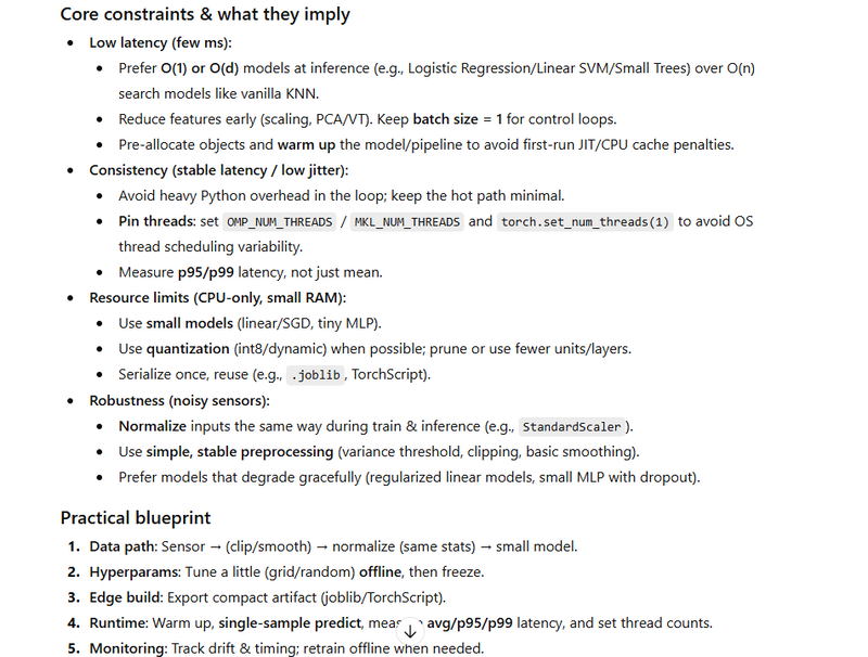
1) Low latency (few ms per prediction)
Pick O(d) models: linear/logistic regression, linear SVM, tiny MLP; avoid heavy ensembles.
Minimize per-sample work: run with batch size = 1, pre-allocate arrays, reuse the same pipeline object.
Warm up: run a few dry predictions at startup to JIT/warm caches and load thread pools.
Keep transforms simple: fixed StandardScaler + VarianceThreshold (no PCA at runtime unless needed).
Cap threads: force BLAS/numexpr/sklearn to 1 thread to avoid context switching spikes for single-sample inference.
2) Consistency (stable latency, not just fast average)
Avoid dynamic work: KNN distance search or big trees can spike; prefer linear models.
Freeze everything: same input dimensionality/order; no optional branches in the hot path.
Use EMA/debouncing (optional) for sensor noise so preprocessing stays stable.
Measure p95/p99 and track deadline misses; treat those as defects.
Preallocate buffers and reuse timers; avoid heap churn in the loop.
3) Resource limits (CPU-only, small RAM)
Shrink features offline: VarianceThreshold, select-K-best.
Compact models: logistic regression with L2, or a tiny MLP; serialize with compression.
Quantization/pruning (when using NN/ONNX/Torch): int8 quantization, prune small weights.
No extra copies: keep data as float32, avoid pandas in the hot loop.
4) Robustness (noisy sensors)
Fixed normalization: fit mean/std on training data; at runtime only apply those constants.
Clamp/outlier guard: clip absurd values to safe ranges before scaling.
Signal smoothing (optional): EMA on inputs or outputs (small α) to prevent control chatter.
Sanity checks: if inputs are NaN or out of plausible range, hold last command or fall back.
Real-time robot control constraints
Low latency: Each prediction must complete within a tight deadline (often a few milliseconds).
Consistency: Stable latency matters as much as average latency—spikes can break control loops.
Resource limits: Edge hardware (CPU-only, small RAM) requires compact, efficient models.
Robustness: Noisy sensors → need normalization and simple, stable preprocessing.
2) Data preprocessing
Normalization (StandardScaler): Keeps features on similar scales so distance-based or gradient-based models behave well; reduces sensitivity to sensor units.
Variance filtering (VarianceThreshold): Drops near-constant features to remove noise and reduce compute.
3) Pipeline construction
Why a Pipeline:
Ensures the exact same transforms are applied at train & inference.
Keeps steps modular and swappable (e.g., change model without touching preprocessing).
Plays nicely with hyperparameter search (you can tune thresholds and model params together).
4) Hyperparameter tuning
GridSearchCV (or RandomizedSearchCV) finds a good configuration under cross-validation:
Accuracy improves.
Indirectly improves latency by letting you pick simpler configurations (e.g., fewer neighbors in KNN) when accuracy stays acceptable.
5) Measuring latency correctly
Warm-up: Do a few predictions first (JIT, caches, CPU frequency ramp-up).
Per-sample latency: Loop one sample at a time (this matches control-loop usage).
Distribution metrics: Track mean and p95 (outliers matter in real-time systems).
6) Model optimization (edge/embedded)
Pruning/Quantization (conceptual here): Reduce size & arithmetic precision to speed up inference and shrink memory footprint.
Feature count: Fewer features → faster scaler + model compute.
Algorithm choice: KNN is simple but can be slower at inference for large datasets (it compares to many points). For bigger problems, consider tree-based models or linear models, or approximate neighbors. For this toy demo, KNN is fine.
7) Production hygiene
Export the fitted pipeline (preprocessing + model) as one artifact.
Version & config control.
Streaming integration: In practice, wrap .predict() in your sensor loop; avoid per-call allocations; reuse buffers if possible.
# =========================
# Real-time ML Pipeline Demo
# =========================
# Goals:
# - Clean, modular sklearn Pipeline
# - CV hyperparameter tuning
# - Inference latency measurement (with warm-up)
# - Simple "optimization" placeholder to illustrate where quantization/pruning would go
# - Save the final pipeline for production use

import time
import numpy as np
import warnings

from sklearn.datasets import load_iris
from sklearn.model_selection import train_test_split, GridSearchCV
from sklearn.pipeline import Pipeline
from sklearn.preprocessing import StandardScaler
from sklearn.feature_selection import VarianceThreshold
from sklearn.neighbors import KNeighborsClassifier
from sklearn.metrics import accuracy_score
from joblib import dump

warnings.filterwarnings("ignore", category=UserWarning)

# -------------------------
# 1) Simulated optimization
# -------------------------
def optimize_model_for_inference(model):
    """
    Placeholder for pruning/quantization/weight-sharing.
    In real systems, you might:
      - Quantize weights/activations (e.g., to int8/float16) with a supported library
      - Prune unimportant parameters (for NN models)
      - Export to ONNX / TensorRT / OpenVINO / TVM and compile for edge hardware
    """
    print("[Optimize] Applying (simulated) model size reduction techniques (pruning/quantization)")
    return model  # No-op here; replace with real optimization when applicable.


# -------------------------
# 2) Load & split data
# -------------------------
# Using Iris as a stand-in for robot sensor vectors.
data = load_iris()
X, y = data.data, data.target

# In robotics, you'd typically have a chronological split; here we use a random split for simplicity.
X_train, X_test, y_train, y_test = train_test_split(
    X, y, test_size=0.2, random_state=42, stratify=y
)


# -------------------------
# 3) Build pipeline
# -------------------------
pipeline = Pipeline([
    ("scaler", StandardScaler()),          # Robustness against scale differences
    ("selector", VarianceThreshold()),     # Drop near-constant features
    ("clf", KNeighborsClassifier())        # Simple classifier (distance-based)
])


# -------------------------
# 4) Define search space
# -------------------------
param_grid = {
    "selector__threshold": [0.0, 0.001, 0.01],
    "clf__n_neighbors": [1, 3, 5, 7],
    "clf__leaf_size": [10, 20, 30],
    "clf__p": [1, 2]  # Manhattan vs Euclidean
}

# -------------------------
# 5) Hyperparameter tuning
# -------------------------
search = GridSearchCV(
    estimator=pipeline,
    param_grid=param_grid,
    cv=3,
    n_jobs=-1,
    scoring="accuracy",
    verbose=1
)
search.fit(X_train, y_train)

best_pipeline = search.best_estimator_
print("\n[Search] Best params:", search.best_params_)
print("[Search] Best CV score: {:.4f}".format(search.best_score_))


# ---------------------------------------------------
# 6) "Optimize" the model & reinsert into the pipeline
# ---------------------------------------------------
optimized_model = optimize_model_for_inference(best_pipeline.named_steps["clf"])
best_pipeline.named_steps["clf"] = optimized_model


# --------------------------------------------
# 7) Evaluate accuracy and measure real-time lat
# --------------------------------------------
# (A) Batch accuracy
y_pred = best_pipeline.predict(X_test)
acc = accuracy_score(y_test, y_pred)
print("\n[Eval] Test Accuracy: {:.2f}%".format(acc * 100.0))

# (B) Warm-up (important to stabilize caches and frequency scaling)
def warmup(pipeline, sample, runs=5):
    for _ in range(runs):
        _ = pipeline.predict(sample.reshape(1, -1))

warmup(best_pipeline, X_test[0], runs=5)

# (C) Per-sample latency measurement (simulate control-loop usage)
def measure_per_sample_latency(pipeline, X, repeats=1):
    """
    Measures per-sample latency (ms) over a sequence of samples.
    repeats: how many times to loop the same stream (to gather more statistics).
    Returns: list of latencies in milliseconds.
    """
    latencies_ms = []
    for _ in range(repeats):
        for i in range(len(X)):
            x = X[i].reshape(1, -1)
            t0 = time.perf_counter()
            _ = pipeline.predict(x)
            t1 = time.perf_counter()
            latencies_ms.append((t1 - t0) * 1000.0)
    return latencies_ms

latencies = measure_per_sample_latency(best_pipeline, X_test, repeats=3)
lat_mean = float(np.mean(latencies))
lat_p95  = float(np.percentile(latencies, 95))
lat_max  = float(np.max(latencies))

print("[Latency] per-sample mean: {:.3f} ms | p95: {:.3f} ms | max: {:.3f} ms".format(
    lat_mean, lat_p95, lat_max
))

# (D) Throughput (optional, for batch scenarios)
def measure_throughput(pipeline, X, batch_size=16, runs=20):
    """
    Measures approximate throughput (samples/sec) with mini-batches.
    """
    # Make sure X length >= batch_size for a fair measure
    if len(X) < batch_size:
        reps = int(np.ceil(batch_size / len(X)))
        Xb = np.tile(X, (reps, 1))[:batch_size]
    else:
        Xb = X[:batch_size]

    # Warm-up batch
    _ = pipeline.predict(Xb)

    t0 = time.perf_counter()
    for _ in range(runs):
        _ = pipeline.predict(Xb)
    t1 = time.perf_counter()

    total_samples = batch_size * runs
    elapsed = t1 - t0
    samples_per_sec = total_samples / elapsed if elapsed > 0 else float('inf')
    return samples_per_sec

tput = measure_throughput(best_pipeline, X_test, batch_size=16, runs=50)
print("[Throughput] ~{:.1f} samples/sec (batch=16)\n".format(tput))

# -------------------------
# 8) Save the final artifact
# -------------------------
artifact_path = "robot_realtime_pipeline.joblib"
dump(best_pipeline, artifact_path)
print("[Export] Saved fitted pipeline (preprocessing + model) to:", artifact_path)

# -------------------------
# 9) Quick sanity prediction
# -------------------------
sample = X_test[0].reshape(1, -1)
pred_class = best_pipeline.predict(sample)[0]
print("[Sanity] Single-sample prediction:", pred_class)
EXPLANATION
Step-by-step: what each block does & why it helps real-time
1) Data load & split
data = load_iris()
X_train, X_test, y_train, y_test = train_test_split(...)
Treats Iris as proxy sensor data. In robots you’d feed IMU/LiDAR/encoder features instead.
The split simulates “past data for training” vs “future/online data for evaluation.”
2) Pipeline definition
pipeline = Pipeline([
  ('scaler', StandardScaler()),
  ('selector', VarianceThreshold()),
  ('classifier', KNeighborsClassifier())
])
StandardScaler: centers/normalizes features so distances & gradients behave sensibly. Vital for KNN and many linear models.
VarianceThreshold: removes features that barely change → reduces noise + dimension → faster inference.
KNN: simple, non-parametric. OK for demos, but you’ll often prefer faster, fixed-cost models in real-time (more below).
3) Joint hyperparameter search
param_grid = {
  'selector__threshold': [0, 0.001, 0.01],
  'classifier__n_neighbors': [1, 3, 5, 7],
  'classifier__leaf_size': [10, 20, 30],
  'classifier__p': [1, 2]
}
grid_search = GridSearchCV(pipeline, param_grid, cv=3, n_jobs=2, verbose=1)
grid_search.fit(X_train, y_train)
Tunes preprocessing + model together → avoids mismatch (e.g., a selector that hurts the chosen model).
cv=3 controls variance of the estimate; n_jobs=2 speeds up the search on CPU.
Output is the best full pipeline, not just best classifier.
4) “Optimize model” placeholder
def optimize_model_for_inference(model):
    print("Applying model size reduction techniques (pruning/quantization)")
    return model
In scikit-learn, true pruning/quantization is limited. This is a hook where you’d:
Export to ONNX → run with ONNX Runtime for CPU vectorization.
Or switch to a framework/model that supports quantization (e.g., PyTorch → QAT, or XGBoost with fast predictors).
5) Latency measurement
start_time = time.time()
y_pred = best_pipeline.predict(X_test)
end_time = time.time()
latency = (end_time - start_time) / len(X_test)
Gives avg per-sample latency—good first approximation for control-loop budgets.
For stricter real-time: warm up first, time per single sample, and measure 95p/99p tail latency.
FULL CODING
# real_time_robot_pipeline.py
import os
import time
import math
import numpy as np
from collections import deque
# Force single-threaded math for stable latency
os.environ["OMP_NUM_THREADS"] = "1"
os.environ["OPENBLAS_NUM_THREADS"] = "1"
os.environ["MKL_NUM_THREADS"] = "1"
os.environ["VECLIB_MAXIMUM_THREADS"] = "1"
os.environ["NUMEXPR_NUM_THREADS"] = "1"
from threadpoolctl import threadpool_limits
from sklearn.datasets import load_iris
from sklearn.model_selection import train_test_split, GridSearchCV
from sklearn.pipeline import Pipeline
from sklearn.preprocessing import StandardScaler
from sklearn.feature_selection import VarianceThreshold
from sklearn.linear_model import LogisticRegression
from sklearn.metrics import accuracy_score
from sklearn.utils.validation import check_is_fitted
import joblib
import warnings
warnings.filterwarnings("ignore", category=UserWarning)
# ---------- Utility: robust percentiles ----------
def percentile(a, q):
if len(a) == 0:
return float("nan")
return float(np.percentile(a, q))
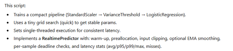
# ---------- Real-time helper (EMA smoothing, clipping, deadline checks) ----------
class RealtimePredictor:
def __init__(self, fitted_pipeline, feature_clip=(-10.0, 10.0), ema_alpha=None, warmup=10, deadline_ms=3.0):
"""
fitted_pipeline: sklearn Pipeline (already .fit())
feature_clip: (min, max) clamp before scaling to guard outliers
ema_alpha: None or float in (0,1]; if set, applies EMA on inputs
warmup: number of dry runs to stabilize caches
deadline_ms: per-sample deadline in milliseconds
"""
self.pipe = fitted_pipeline
check_is_fitted(self.pipe)
self.clip_min, self.clip_max = feature_clip
self.ema_alpha = ema_alpha
self.deadline_ms = float(deadline_ms)
# Determine input dimensionality from the scaler
scaler = self.pipe.named_steps["scaler"]
self.n_features = scaler.scale_.shape[0]
# Preallocate a 2D array for single-sample predict (shape must be (1, d))
self._buf = np.empty((1, self.n_features), dtype=np.float32)
# EMA state
self._ema = None
# Warm-up: use training means (zeros after scaling) as dummy input
dummy = np.zeros((1, self.n_features), dtype=np.float32)
for _ in range(max(0, int(warmup))):
_ = self.pipe.predict(dummy)
# Stats
self.latencies_ms = []
self.deadline_misses = 0
self.total = 0
def _preprocess(self, x1d):
"""Clamp, optional EMA, and copy into the preallocated buffer."""
z = np.asarray(x1d, dtype=np.float32)
if z.ndim != 1 or z.shape[0] != self.n_features:
raise ValueError(f"Expected 1D feature array of length {self.n_features}, got {z.shape}")
# Clip outliers
np.clip(z, self.clip_min, self.clip_max, out=z)
# EMA smoothing (on raw features, before scaling)
if self.ema_alpha is not None:
if self._ema is None:
self._ema = z.copy()
else:
self._ema = self.ema_alpha * z + (1.0 - self.ema_alpha) * self._ema
z = self._ema
# Place into preallocated buffer (as a row)
self._buf[0, :] = z
return self._buf # shape (1, d)
def predict_one(self, x1d):
"""
Returns: (pred, latency_ms, deadline_met: bool)
"""
xrow = self._preprocess(x1d)
t0 = time.perf_counter()
y = self.pipe.predict(xrow)
t1 = time.perf_counter()
lat_ms = (t1 - t0) * 1000.0
self.total += 1
self.latencies_ms.append(lat_ms)
met = lat_ms <= self.deadline_ms
if not met:
self.deadline_misses += 1
return int(y[0]), lat_ms, met
def report(self):
lat = self.latencies_ms
return {
"count": len(lat),
"avg_ms": float(np.mean(lat)) if lat else float("nan"),
"p95_ms": percentile(lat, 95),
"p99_ms": percentile(lat, 99),
"max_ms": max(lat) if lat else float("nan"),
"deadline_ms": self.deadline_ms,
"misses": self.deadline_misses,
"miss_rate": (self.deadline_misses / max(1, self.total)) * 100.0,
}
# ---------- Training + small grid search (fast, stable) ----------
def train_compact_pipeline(X_train, y_train):
base = Pipeline([
("scaler", StandardScaler(with_mean=True, with_std=True)),
("selector", VarianceThreshold()), # cheap dimensionality drop
("clf", LogisticRegression(
penalty="l2",
solver="lbfgs", # stable on small/medium dims
max_iter=500,
n_jobs=1, # explicit
)),
])
# Tiny search space to keep it fast and predictable
grid = {
"selector__threshold": [0.0, 0.001, 0.01],
"clf__C": [0.5, 1.0, 2.0],
"clf__tol": [1e-4, 1e-3],
}
with threadpool_limits(limits=1):
gs = GridSearchCV(
base, grid, cv=3, n_jobs=1, verbose=0, return_train_score=False
)
gs.fit(X_train, y_train)
best = gs.best_estimator_
return best, gs.best_params_
# ---------- Optional: “size optimization placeholder” ----------
def optimize_for_edge(pipeline):
"""
Placeholder to simulate model compaction steps for edge devices.
Real options (if/when needed): ONNX export + int8 quant, or NN pruning+quant.
Here we just ensure float32 in the hot path and compress the serialized file.
"""
# Ensure downstream uses float32
# (LogReg uses float64 by default internally; we just keep inputs float32)
return pipeline
# ---------- Main demo ----------
def main():
# 1) Load data (proxy for robot sensors)
data = load_iris()
X = data.data.astype(np.float32)
y = data.target
# 2) Split
X_train, X_test, y_train, y_test = train_test_split(
X, y, test_size=0.25, random_state=42, stratify=y
)
# 3) Train compact pipeline
pipeline, best_params = train_compact_pipeline(X_train, y_train)
print("Best hyperparameters:", best_params)
# 4) Edge optimization placeholder
pipeline = optimize_for_edge(pipeline)
# 5) Accuracy sanity check
with threadpool_limits(limits=1):
y_pred = pipeline.predict(X_test)
acc = accuracy_score(y_test, y_pred)
print(f"Holdout accuracy: {acc*100:.2f}%")
# 6) Real-time predictor
# - Clip extremes (depends on your sensors; here, generous bounds)
# - EMA smoothing small (alpha ~ 0.2) to reduce jitter but keep responsiveness
# - Deadline: e.g., 3 ms per sample on CPU (adjust to your target)
predictor = RealtimePredictor(
fitted_pipeline=pipeline,
feature_clip=(-10.0, 10.0),
ema_alpha=0.2, # set None to disable smoothing
warmup=15,
deadline_ms=3.0,
)
# 7) Simulate a streaming loop over test samples (repeat to get stats)
misses = 0
lat_log = deque(maxlen=5) # last 5 latencies, for quick look
repeats = 5 # repeat stream a few times to gather p95/p99
for _ in range(repeats):
for xi, yi in zip(X_test, y_test):
pred, lat_ms, met = predictor.predict_one(xi)
lat_log.append(lat_ms)
if not met:
misses += 1
# In a real robot: convert pred -> control signal here
# Optionally use output smoothing/guards for actuator safety
# 8) Report latency and deadline performance
stats = predictor.report()
print("\nLatency stats (ms):")
print(f" count={stats['count']}, avg={stats['avg_ms']:.3f}, p95={stats['p95_ms']:.3f}, "
f"p99={stats['p99_ms']:.3f}, max={stats['max_ms']:.3f}")
print(f"Deadline: {stats['deadline_ms']:.2f} ms | Misses: {stats['misses']} "
f"({stats['miss_rate']:.2f}%)")
print(f"Recent latencies (last {len(lat_log)}): " + ", ".join(f"{x:.3f}" for x in lat_log))
# 9) Persist model (compressed) for edge deployment
out_path = "robot_control_compact_pipeline.joblib"
joblib.dump(pipeline, out_path, compress=("xz", 3))
print(f"\nSaved compact pipeline to: {out_path}")
if __name__ == "__main__":
main()

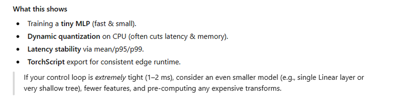
SECOND EXAMPLE
# edge_robot_control.py
# Demo: Optimizing ML for edge-based robot control — latency, stability, efficiency (CPU-only).
# - Small MLP classifier trained on synthetic "sensor" data
# - Robust preprocessing (z-score, clipping, optional EMA)
# - Inference optimizations: no_grad, set_num_threads, TorchScript, dynamic quantization
# - Latency benchmarking with tail stats (p95/p99) and jitter
# - Model size comparison (fp32 vs quantized)

import os
import io
import time
import math
import random
from typing import Tuple, List

import numpy as np
import torch
import torch.nn as nn
import torch.nn.functional as F

# -----------------------
# Repro & CPU settings
# -----------------------
SEED = 42
random.seed(SEED); np.random.seed(SEED); torch.manual_seed(SEED)

# For edge CPUs, fewer threads often => more consistent latency (less OS scheduling jitter)
torch.set_num_threads(1)
torch.set_num_interop_threads(1)

DEVICE = torch.device("cpu")

# -----------------------
# Synthetic "sensor" dataset
#  - 16 features
#  - 3 classes
#  - Add some noise/outliers for robustness testing
# -----------------------
def make_synthetic_data(n_samples=4000, n_features=16, n_classes=3, train_ratio=0.8) -> Tuple[np.ndarray, np.ndarray, np.ndarray, np.ndarray]:
    # Create three cluster centers and sample around them
    centers = np.array([
        np.linspace(-1.0,  1.0, n_features),
        np.linspace( 0.5, -0.5, n_features),
        np.linspace( 1.0,  0.2, n_features)
    ])
    X = []
    y = []
    for i in range(n_samples):
        cls = np.random.randint(0, n_classes)
        vec = centers[cls] + 0.25 * np.random.randn(n_features)
        # inject occasional outliers
        if np.random.rand() < 0.02:
            j = np.random.randint(0, n_features)
            vec[j] += np.random.randn() * 6.0
        X.append(vec); y.append(cls)
    X = np.array(X, dtype=np.float32)
    y = np.array(y, dtype=np.int64)
    idx = np.arange(n_samples)
    np.random.shuffle(idx)
    split = int(train_ratio * n_samples)
    tr, te = idx[:split], idx[split:]
    return X[tr], y[tr], X[te], y[te]

X_train, y_train, X_test, y_test = make_synthetic_data()

# -----------------------
# Robust, cheap preprocessing (fit on train, apply everywhere)
# -----------------------
class Preprocess:
    def __init__(self, mean: np.ndarray, std: np.ndarray, clip: float = 3.0, ema_alpha: float = 0.0):
        self.mean = mean.astype(np.float32)
        self.std = np.maximum(std.astype(np.float32), 1e-6)
        self.clip = float(clip)
        self.ema_alpha = float(ema_alpha)
        self._ema_state = None  # optional smoothing

    @staticmethod
    def fit(X: np.ndarray):
        mean = X.mean(axis=0)
        std  = X.std(axis=0)
        return mean, std

    def _ema(self, x: np.ndarray) -> np.ndarray:
        if self.ema_alpha <= 0.0:
            return x
        if self._ema_state is None:
            self._ema_state = x.copy()
            return x
        self._ema_state = self.ema_alpha * x + (1.0 - self.ema_alpha) * self._ema_state
        return self._ema_state

    def transform(self, x: np.ndarray) -> np.ndarray:
        # x: shape (features,) for single sample
        # z-score
        z = (x - self.mean) / self.std
        # clip outliers
        z = np.clip(z, -self.clip, self.clip)
        # optional EMA smoothing
        z = self._ema(z)
        return z.astype(np.float32)

# Fit preprocessing
mean, std = Preprocess.fit(X_train)
pre = Preprocess(mean, std, clip=3.0, ema_alpha=0.0)  # set ema_alpha>0 (e.g., 0.1) if you want smoothing

# Apply to full sets (training only; online transform happens per-sample at inference)
X_train_p = ((X_train - mean) / np.maximum(std, 1e-6)).clip(-3, 3).astype(np.float32)
X_test_p  = ((X_test  - mean) / np.maximum(std, 1e-6)).clip(-3, 3).astype(np.float32)

# -----------------------
# Small, edge-friendly model
# -----------------------
class SmallMLP(nn.Module):
    def __init__(self, in_dim=16, hidden=32, out_dim=3):
        super().__init__()
        self.fc1 = nn.Linear(in_dim, hidden)
        self.fc2 = nn.Linear(hidden, hidden)
        self.fc3 = nn.Linear(hidden, out_dim)

    def forward(self, x):
        # x: [N, 16]
        x = F.relu(self.fc1(x))
        x = F.relu(self.fc2(x))
        x = self.fc3(x)
        return x

model = SmallMLP().to(DEVICE)

# -----------------------
# Quick training (few epochs)
# -----------------------
def train_quick(model, X, y, epochs=8, batch_size=64, lr=1e-2):
    model.train()
    opt = torch.optim.Adam(model.parameters(), lr=lr)
    X_t = torch.tensor(X, device=DEVICE)
    y_t = torch.tensor(y, device=DEVICE)
    n = X_t.size(0)
    for ep in range(epochs):
        # simple mini-batch loop
        perm = torch.randperm(n)
        total_loss = 0.0
        for i in range(0, n, batch_size):
            idx = perm[i:i+batch_size]
            xb = X_t[idx]
            yb = y_t[idx]
            opt.zero_grad(set_to_none=True)
            logits = model(xb)
            loss = F.cross_entropy(logits, yb)
            loss.backward()
            opt.step()
            total_loss += loss.item() * xb.size(0)
        if (ep+1) % 2 == 0:
            print(f"[train] epoch {ep+1}/{epochs} loss={total_loss/n:.4f}")

train_quick(model, X_train_p, y_train)

# Quick test accuracy (not the main focus; control often uses regression/classification glue)
def accuracy(model, X, y):
    model.eval()
    with torch.no_grad():
        logits = model(torch.tensor(X, device=DEVICE))
        preds = logits.argmax(dim=1).cpu().numpy()
    return (preds == y).mean()

acc_fp32 = accuracy(model, X_test_p, y_test)
print(f"[baseline] FP32 test accuracy: {acc_fp32*100:.2f}%")

# -----------------------
# Export sizes (helper)
# -----------------------
def bytes_of_torch(model_to_save: nn.Module, scripted: bool = False) -> int:
    buf = io.BytesIO()
    if scripted:
        torch.jit.save(model_to_save, buf)
    else:
        torch.save(model_to_save.state_dict(), buf)
    return buf.tell()

# -----------------------
# Baseline eager inference benchmark
# -----------------------
def benchmark_stream(model, pre: Preprocess, X_stream: np.ndarray, warmup=50) -> dict:
    latencies = []
    model.eval()
    # Warmup
    with torch.no_grad():
        for i in range(min(warmup, len(X_stream))):
            x = pre.transform(X_stream[i].copy())
            _ = model(torch.from_numpy(x).unsqueeze(0).to(DEVICE))

    # Timed loop
    with torch.no_grad():
        for i in range(len(X_stream)):
            x = pre.transform(X_stream[i].copy())
            t0 = time.perf_counter()
            out = model(torch.from_numpy(x).unsqueeze(0).to(DEVICE))
            _ = out.argmax(dim=1)
            t1 = time.perf_counter()
            latencies.append((t1 - t0) * 1000.0)  # ms

    lat = np.array(latencies)
    stats = {
        "count": int(lat.size),
        "avg_ms": float(lat.mean()),
        "p50_ms": float(np.percentile(lat, 50)),
        "p95_ms": float(np.percentile(lat, 95)),
        "p99_ms": float(np.percentile(lat, 99)),
        "std_ms": float(lat.std(ddof=1)),
    }
    return stats

X_stream = X_test  # raw test samples; preprocess applied inside benchmark

print("\n[benchmark] Baseline (FP32 eager)")
base_stats = benchmark_stream(model, pre, X_stream, warmup=50)
for k, v in base_stats.items():
    print(f"  {k}: {v:.4f}" if isinstance(v, float) else f"  {k}: {v}")

base_size = bytes_of_torch(model, scripted=False)
print(f"  model_size_bytes (state_dict): {base_size}")

# -----------------------
# Optimization 1: TorchScript (script) to cut Python overhead
# -----------------------
scripted_model = torch.jit.script(model.eval())
print("\n[benchmark] TorchScript (FP32)")
ts_stats = benchmark_stream(scripted_model, pre, X_stream, warmup=50)
for k, v in ts_stats.items():
    print(f"  {k}: {v:.4f}" if isinstance(v, float) else f"  {k}: {v}")
ts_size = bytes_of_torch(scripted_model, scripted=True)
print(f"  model_size_bytes (torchscript): {ts_size}")

# -----------------------
# Optimization 2: Dynamic quantization (int8 Linear) + TorchScript
#   - Great for CPU + Linear/LSTM heavy nets
# -----------------------
quantized = torch.quantization.quantize_dynamic(
    model.eval(),
    {nn.Linear},  # quantize all Linear layers
    dtype=torch.qint8
)
scripted_quant = torch.jit.script(quantized.eval())

# Accuracy check after quantization
acc_q = accuracy(quantized, X_test_p, y_test)
print(f"\n[quant] quantized test accuracy: {acc_q*100:.2f}%")

print("\n[benchmark] TorchScript + Dynamic Quant (INT8 Linear)")
q_stats = benchmark_stream(scripted_quant, pre, X_stream, warmup=50)
for k, v in q_stats.items():
    print(f"  {k}: {v:.4f}" if isinstance(v, float) else f"  {k}: {v}")
q_size = bytes_of_torch(scripted_quant, scripted=True)
print(f"  model_size_bytes (torchscript+quant): {q_size}")

# -----------------------
# Summary
# -----------------------
def pct(a, b):
    return 100.0 * (a - b) / max(a, 1e-9)

print("\n=== SUMMARY (lower is better) ===")
print(f"Accuracy FP32      : {acc_fp32*100:.2f}%")
print(f"Accuracy Quantized : {acc_q*100:.2f}%")
print(f"Avg latency  FP32 eager       : {base_stats['avg_ms']:.4f} ms")
print(f"Avg latency  TorchScript FP32 : {ts_stats['avg_ms']:.4f} ms ({pct(base_stats['avg_ms'], ts_stats['avg_ms']):+.1f}% vs FP32 eager)")
print(f"Avg latency  TS + Quant INT8  : {q_stats['avg_ms']:.4f} ms ({pct(base_stats['avg_ms'], q_stats['avg_ms']):+.1f}% vs FP32 eager)")
print(f"p95   FP32 eager       : {base_stats['p95_ms']:.4f} ms")
print(f"p95   TorchScript FP32 : {ts_stats['p95_ms']:.4f} ms")
print(f"p95   TS + Quant INT8  : {q_stats['p95_ms']:.4f} ms")
print(f"Jitter (std) FP32 eager: {base_stats['std_ms']:.4f} ms")
print(f"Jitter (std) TS+Quant  : {q_stats['std_ms']:.4f} ms")
print(f"Model size (state_dict)         : {base_size} bytes")
print(f"Model size (TorchScript FP32)   : {ts_size} bytes")
print(f"Model size (TorchScript INT8)   : {q_size} bytes")

# -----------------------
# How to deploy on edge (notes):
# 1) Keep torch.set_num_threads(1) for predictability; consider taskset/CPU affinity at OS level.
# 2) Pre-allocate tensors if possible; avoid per-call allocations.
# 3) Fixed-length inputs and simple control branches.
# 4) Log and watch p95/p99 in production; alert on spikes/drift.
# -----------------------
ML EXAMPLE
# ====== classical_ml_edge_pipeline.py ======
import os
import time
import numpy as np
from pathlib import Path

from sklearn.datasets import load_iris
from sklearn.model_selection import train_test_split, GridSearchCV
from sklearn.pipeline import Pipeline
from sklearn.preprocessing import StandardScaler
from sklearn.feature_selection import VarianceThreshold
from sklearn.decomposition import PCA
from sklearn.linear_model import SGDClassifier
from sklearn.metrics import accuracy_score
import joblib

# -----------------------------
# 0) (Optional) make CPU timing more stable
# -----------------------------
os.environ["OMP_NUM_THREADS"] = "1"
os.environ["MKL_NUM_THREADS"] = "1"

# -----------------------------
# 1) Load data (proxy for sensors)
# -----------------------------
data = load_iris()
X, y = data.data, data.target

# Add a touch of noise to mimic sensors
rng = np.random.default_rng(42)
X = X + rng.normal(0, 0.01, X.shape)

X_train, X_test, y_train, y_test = train_test_split(
    X, y, test_size=0.2, random_state=42, stratify=y
)

# -----------------------------
# 2) Compact, stable pipeline
#    - Standardize
#    - Drop low-variance features
#    - PCA to reduce dimensionality (speeds up inference, stabilizes)
#    - Linear model (SGDClassifier) ~ O(d) per inference
# -----------------------------
pipe = Pipeline([
    ("scaler", StandardScaler(with_mean=True, with_std=True)),
    ("vt", VarianceThreshold(threshold=0.0)),
    ("pca", PCA(n_components=2, svd_solver="auto", random_state=42)),
    ("clf", SGDClassifier(loss="log_loss", penalty="l2", max_iter=300, tol=1e-3, random_state=42))
])

# -----------------------------
# 3) Light hyperparameter tuning (small grid)
# -----------------------------
param_grid = {
    "pca__n_components": [2, 3],
    "clf__alpha": [1e-4, 1e-3, 1e-2],
}
gs = GridSearchCV(pipe, param_grid, cv=3, n_jobs=1, verbose=0)
gs.fit(X_train, y_train)
best = gs.best_estimator_

print("Best params:", gs.best_params_)

# -----------------------------
# 4) Evaluate accuracy
# -----------------------------
y_pred = best.predict(X_test)
acc = accuracy_score(y_test, y_pred)
print(f"Test Accuracy: {acc*100:.2f}%")

# -----------------------------
# 5) Warm-up + latency measurement (single-sample)
# -----------------------------
def measure_latency(model, X_samples, runs=1000):
    # Warm-up
    for _ in range(50):
        _ = model.predict(X_samples[0:1])

    times = []
    for i in range(runs):
        x = X_samples[i % len(X_samples): (i % len(X_samples)) + 1]
        t0 = time.perf_counter()
        _ = model.predict(x)
        t1 = time.perf_counter()
        times.append((t1 - t0) * 1000.0)  # ms

    times = np.array(times)
    return {
        "mean_ms": float(times.mean()),
        "p95_ms": float(np.percentile(times, 95)),
        "p99_ms": float(np.percentile(times, 99)),
        "min_ms": float(times.min()),
        "max_ms": float(times.max()),
    }

lat_stats = measure_latency(best, X_test, runs=1000)
print("Latency (ms) single sample:", lat_stats)

# -----------------------------
# 6) Save compact artifact
# -----------------------------
out_dir = Path("artifacts_ml")
out_dir.mkdir(exist_ok=True)
joblib.dump(best, out_dir / "edge_linear_pipeline.joblib")
print(f"Saved: {out_dir / 'edge_linear_pipeline.joblib'}")

# -----------------------------
# 7) Example: edge runtime load + predict
# -----------------------------
loaded = joblib.load(out_dir / "edge_linear_pipeline.joblib")
sample_pred = loaded.predict(X_test[0:1])
print("Edge runtime sample prediction:", sample_pred)
DEEP LEARNING EXAMPLE
# ====== tiny_dl_edge_pipeline.py ======
import os
import time
import numpy as np

import torch
import torch.nn as nn
import torch.optim as optim
from sklearn.model_selection import train_test_split

# -----------------------------
# 0) Make CPU timing more stable
# -----------------------------
os.environ["OMP_NUM_THREADS"] = "1"
os.environ["MKL_NUM_THREADS"] = "1"
torch.set_num_threads(1)

DEVICE = torch.device("cpu")

# -----------------------------
# 1) Create synthetic sensor-like dataset
#    (You would replace this with real sensor frames.)
# -----------------------------
rng = np.random.default_rng(1)
N = 1200
D = 16  # feature dimension
C = 3   # classes

X = rng.normal(0, 1.0, size=(N, D)).astype(np.float32)
# Create a simple non-linear label rule
W_true = rng.normal(0, 1.0, size=(D, C)).astype(np.float32)
y = np.argmax(np.tanh(X @ W_true) + 0.05 * rng.normal(0, 1.0, size=(N, C)), axis=1).astype(np.int64)

# Normalize like a scaler (mean/std from train split)
X_train, X_test, y_train, y_test = train_test_split(X, y, stratify=y, test_size=0.2, random_state=42)
mean = X_train.mean(axis=0, keepdims=True)
std = X_train.std(axis=0, keepdims=True) + 1e-6
X_train = (X_train - mean) / std
X_test = (X_test - mean) / std

X_train_t = torch.from_numpy(X_train)
y_train_t = torch.from_numpy(y_train)
X_test_t = torch.from_numpy(X_test)
y_test_t = torch.from_numpy(y_test)

# -----------------------------
# 2) Tiny MLP model (edge-friendly)
# -----------------------------
class TinyMLP(nn.Module):
    def __init__(self, in_dim=16, hidden=32, out_dim=3, p_drop=0.1):
        super().__init__()
        self.net = nn.Sequential(
            nn.Linear(in_dim, hidden),
            nn.ReLU(inplace=True),
            nn.Dropout(p_drop),
            nn.Linear(hidden, out_dim)
        )

    def forward(self, x):
        return self.net(x)

model = TinyMLP(in_dim=D, hidden=32, out_dim=C, p_drop=0.1).to(DEVICE)

# -----------------------------
# 3) Train briefly (CPU)
# -----------------------------
criterion = nn.CrossEntropyLoss()
optimizer = optim.Adam(model.parameters(), lr=1e-3)
model.train()

epochs = 12
batch_size = 64
for epoch in range(epochs):
    # mini-batch training
    perm = torch.randperm(len(X_train_t))
    X_train_t = X_train_t[perm]
    y_train_t = y_train_t[perm]

    for i in range(0, len(X_train_t), batch_size):
        xb = X_train_t[i:i+batch_size].to(DEVICE)
        yb = y_train_t[i:i+batch_size].to(DEVICE)

        optimizer.zero_grad(set_to_none=True)
        logits = model(xb)
        loss = criterion(logits, yb)
        loss.backward()
        optimizer.step()

    if (epoch+1) % 4 == 0:
        with torch.no_grad():
            logits = model(torch.from_numpy(X_test).to(DEVICE))
            preds = logits.argmax(dim=1).cpu().numpy()
            acc = (preds == y_test).mean()
        print(f"Epoch {epoch+1:02d}: loss={loss.item():.4f}, test_acc={acc*100:.2f}%")

# -----------------------------
# 4) Baseline FP32 latency (single-sample)
# -----------------------------
def latency_stats(predict_fn, X_np, runs=1000):
    # Warm-up
    for _ in range(50):
        _ = predict_fn(X_np[0:1])

    times = []
    for i in range(runs):
        x = X_np[i % len(X_np): (i % len(X_np)) + 1]
        t0 = time.perf_counter()
        _ = predict_fn(x)
        t1 = time.perf_counter()
        times.append((t1 - t0) * 1000.0)  # ms
    ts = np.array(times)
    return {
        "mean_ms": float(ts.mean()),
        "p95_ms": float(np.percentile(ts, 95)),
        "p99_ms": float(np.percentile(ts, 99)),
        "min_ms": float(ts.min()),
        "max_ms": float(ts.max()),
    }

@torch.no_grad()
def predict_fp32(x_np):
    x = torch.from_numpy(x_np.astype(np.float32)).to(DEVICE)
    out = model(x)
    return out.argmax(dim=1).cpu().numpy()

fp32_stats = latency_stats(predict_fp32, X_test, runs=1000)
print("FP32 latency (ms):", fp32_stats)

# -----------------------------
# 5) Dynamic quantization (int8 weights for Linear)
#    - Very effective on CPU for Linear/LSTM layers
# -----------------------------
quantized = torch.quantization.quantize_dynamic(
    model, {nn.Linear}, dtype=torch.qint8
).to(DEVICE).eval()

@torch.no_grad()
def predict_int8(x_np):
    x = torch.from_numpy(x_np.astype(np.float32)).to(DEVICE)
    out = quantized(x)
    return out.argmax(dim=1).cpu().numpy()

int8_stats = latency_stats(predict_int8, X_test, runs=1000)
print("INT8 (dynamic) latency (ms):", int8_stats)

# -----------------------------
# 6) Accuracy check after quantization
# -----------------------------
with torch.no_grad():
    acc_fp32 = (predict_fp32(X_test) == y_test).mean()
    acc_int8 = (predict_int8(X_test) == y_test).mean()
print(f"Accuracy FP32: {acc_fp32*100:.2f}% | INT8: {acc_int8*100:.2f}%")

# -----------------------------
# 7) Optional: TorchScript export for stable edge runtime
# -----------------------------
example = torch.from_numpy(X_test[0:1].astype(np.float32)).to(DEVICE)
traced = torch.jit.trace(quantized, example)
torch.jit.save(traced, "artifacts_dl_tiny_mlp_int8.pt")
print("Saved TorchScript model: artifacts_dl_tiny_mlp_int8.pt")

# -----------------------------
# 8) Edge runtime hot path example (TorchScript)
# -----------------------------
loaded_ts = torch.jit.load("artifacts_dl_tiny_mlp_int8.pt", map_location=DEVICE)
loaded_ts.eval()

@torch.no_grad()
def predict_ts(x_np):
    x = torch.from_numpy(x_np.astype(np.float32)).to(DEVICE)
    out = loaded_ts(x)
    return out.argmax(dim=1).cpu().numpy()

ts_stats = latency_stats(predict_ts, X_test, runs=1000)
print("TorchScript INT8 latency (ms):", ts_stats)

Top comments (0)